At work I have been playing with Jev by TypeSafe AI a lot, and the reason it got popular is pretty s 2026-9-29 06:50:23 Author: hackernoon.com(查看原文) 阅读量:2 收藏
At work I have been playing with Jev by TypeSafe AI a lot, and the reason it got popular is pretty straightforward: it opened up a class of possibilities where you get an intelligent, LLM-like model that doesn't take forever, so you can use it as a quick classifier for actions -- typed choices, scores, or yes/no probabilities that your software can act on directly, instead of waiting on a long autoregressive reply. That speed is useful, and it also changes how features fail if you ship the score the wrong way.
Speed x quality
LLMs are slow, but they can reason in text. Jev is fast, and what you get back is uncertainty as numbers -- in spirit that sits closer to cross-encoders and other classifiers that read text and emit probabilities over labels, where the model understands the input and then gives you a distribution you can threshold. The difference vs older BERT-style task models is that Jev is trained across a much wider set of decision-shaped work, so the output isn't locked to one fixed label set you trained yourself. ML teams normally ship models that are specific to a task -- one model for fraud prediction, another for product categorization, another for intent, and so on -- because having the model specialize on a certain task usually beats asking one general model to do many things.
What Jev introduces is generalization in that slot: the same underlying Jev model can be asked a lot of different decision shapes across your product. That is useful, and it is also why you have to be careful -- you need to know whether it is actually good at your particular task at all. You can look at how the TypeSafe team talks about benchmarking and calibration, but it is even better to see it on your own data before you let the score decide anything important.
Probabilities change how you work with it
With a lot of LLM apps, you can often ship a prompt, watch a few traces, and feel like it mostly works for the use case. Failures are messy, but they show up as bad text you can read and patch.
Because Jev gives probabilities, your way of working with it is different. There is a higher chance it gets something wrong, or is not confident enough in the answer, and a bare threshold will still fire -- so you need to know when it fails. To learn the model's weakness on your distribution, benchmark it for your use case with offline evals, ideally on your own data from real user interactions with the product.
Whether or not you have "enough" data for an eval is also a concern when you pursue this; it ultimately depends on your use case and how niche your product's data is. A generic support-intent problem is easier to approximate than a workflow only your own customers use. In practice I normally think about three different paths, and they all end in the same place: a labeled set you can score, then a ship decision that still leaves room for a fallback when Jev is unsure.
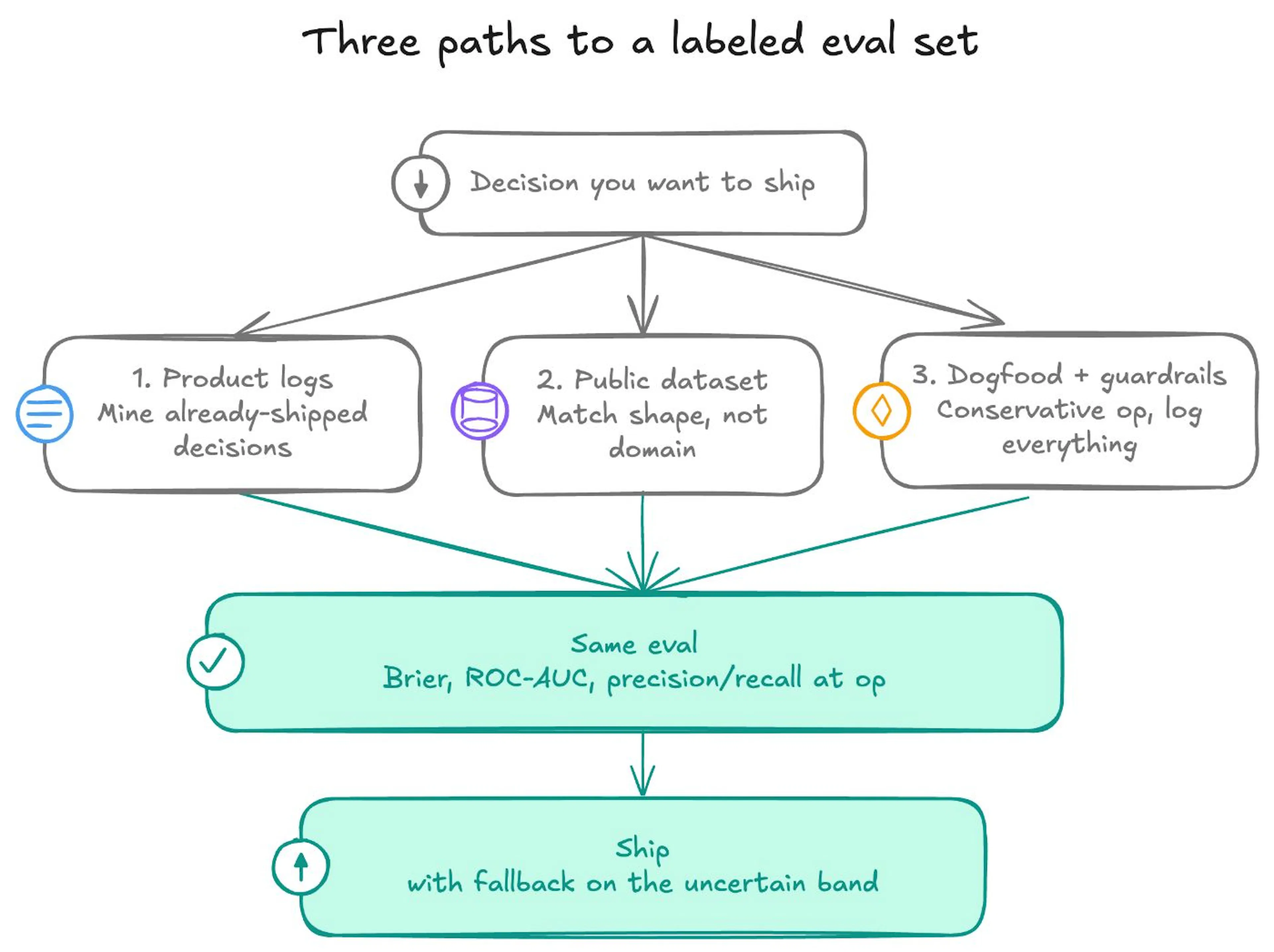 Figure: three ways to build a labeled set -- product logs, a shape-matched public dataset, or dogfood with guardrails -- all feeding the same eval before you ship with a fallback.
Start with the decision you actually want to put in production -- escalate or not, spam or not, which support bucket, or whether a chunk is relevant -- and from there pick whichever path can get you labels fastest.
The first path is mining your own product. If you already have humans or LLMs making that decision in the wild, those outcomes can be used as free labels: you log the same inputs you would send Jev, run Jev offline against that decision, and ask whether the fast model reproduces a call you already trusted enough to ship.
The second path is a public dataset that matches the shape of the decision. A customer sentiment router can dry-run on something like banking77; a spam filter can dry-run on a spam corpus; an agent retrieval step can dry-run on MS MARCO-style relevance. You are testing whether your eval pipeline and metrics make sense, not proving your niche traffic is covered.
The third path is when you have almost nothing: dogfood, beta, or a tight A/B, with a conservative operating point and logging on every call -- you are buying labels with careful exposure instead of with history.
Whatever path you use, they all land on the same final step: evaluate on that labeled set before you trust the score in production, keep a fallback for the uncertain band, and only then put traffic on the cheaper path.
Acquiring samples from your product for an eval
The cheapest place to start is a decision your product already makes by hand or with a slower LLM. You treat those past decisions as ground truth -- a labeled set -- and check whether Jev would have made the same call.
Take support-inbox triage. A ticket comes in: "I was charged twice for March." Someone on the team (or an LLM already in the pipeline) has to put it in a bucket -- {billing, bug, account, other} -- and maybe also decide when to escalate to a human versus handle it itself. That output is essentially a label: it is the answer you already trusted enough to show a customer or hand to an agent. If you save the ticket text and that answer together, you have a free example for eval.
You would then want to log a few weeks of traffic to build out samples for your dataset. For each ticket, store what Jev would see later: subject, body, and any metadata the router uses (plan tier, which product the person is on, whether they are enterprise, how many tickets they have opened before). Then, on an offline evaluation run -- not in front of customers -- run Jev on that same log with the question you want in production, for example "which of these four buckets?" or "should this escalate?" where Jev would return probabilities over the possible support ticket buckets or whether or not the ticket should be escalated. You would then pick the top bucket where Jev returns the highest probabilities, or you turn "escalate" into a yes/no via a probability cutoff, and you compare that to the saved label.
ticket                              human label   Jev (top probs)              what you'd do
---------------------------------------------------------------------------------------------
"I was charged twice for March."    billing       billing 0.82, account 0.11   auto-route (match, high conf)
"Can't log in after password reset" bug           account 0.70, bug 0.18       do not auto-route (confident miss)
"Weird charge + login error today"  ? / messy     billing 0.41, bug 0.39       fallback to human/LLM (uncertain)
Once you have labels, you need more than one score that "passes." Start with Brier score for calibration and overconfidence -- there is no universal good number, lower is better, and this is why recording it matters: it gives you a baseline for how well calibrated the model is, so when you evaluate another model, threshold policy, or cascade on the same benchmark, you can compare relative to that baseline and know not only whether the model is accurate, but also whether you can trust the numbers it gives. After that you still need business-facing accuracy (precision and recall at a cutoff) and a ranking check that does not depend on any one cutoff. The walkthrough below covers calibration first, then those accuracy and ranking pieces.
A quick Brier walkthrough
For a binary decision (escalate vs not, spam vs not, relevant vs not), if p is the model's predicted probability of the positive class and y is the label (1 or 0), the per-example squared error and the Brier score over N examples are:
error_i = (p_i - y_i)^2

Brier = (1/N) * sum_i (p_i - y_i)^2
So Brier is just mean squared error on probabilities: perfect forecasts give 0, always predicting 0.5 on a balanced set lands around 0.25, and being confidently wrong hurts a lot more than being uncertain. Punishing overconfidence is important when you roll these kinds of models out to production, because a model that is wrong at 0.9 is much more dangerous to auto-act on than a model that is unsure at 0.55, even if both look similar after you turn the scores into yes/no.
Here is a tiny numerical example. Suppose you logged four escalate decisions from product traffic:
# p = P(escalate), y = what actually happened (1 = escalated)
ex1: p=0.90, y=1  -> (0.90 - 1)^2 = 0.01   # confident and right
ex2: p=0.80, y=0  -> (0.80 - 0)^2 = 0.64   # confident and wrong (overconfident)
ex3: p=0.55, y=1  -> (0.55 - 1)^2 = 0.2025 # unsure, happened to be right
ex4: p=0.20, y=0  -> (0.20 - 0)^2 = 0.04   # low score, correctly not escalate

Brier = (0.01 + 0.64 + 0.2025 + 0.04) / 4
      = 0.8925 / 4
      = 0.223
You can see that most of that score is contributed by ex2, where the model was overconfidently wrong. The miss was not just a wrong label after thresholding, but it was rather a high-p miss, which is exactly the failure mode that burns you when you auto-act on high confidence. When you compare that to a more conservative model on the same four labels:
ex1: p=0.70, y=1  -> 0.09
ex2: p=0.40, y=0  -> 0.16
ex3: p=0.60, y=1  -> 0.16
ex4: p=0.25, y=0  -> 0.0625

Brier = (0.09 + 0.16 + 0.16 + 0.0625) / 4 = 0.118125
You can see that Brier score for the conservative model is 2x lower, even though both models can still be thresholded into similar yes/no behavior. Recording this Brier score is thus pretty important; it essentially gives you a baseline for how calibrated the model is, so that when you need to evaluate how another model performs on the same benchmark, you can compare relative to that baseline to know if you can trust the numbers that it gives.
If the decision the model needs to give is multiclass (for example, sorting into customer support ticket categories of {billing, bug, account, other}), the usual form is mean squared error over the full probability vector versus a one-hot label:
# p_ik = predicted prob for class k on example i
# y_ik = 1 if label is class k, else 0
# K = number of classes

Brier = (1/N) * sum_i sum_k (p_ik - y_ik)^2
Same idea as the binary case: if you put most of the probability on the wrong class, the squared error is large, and if you spread probability because you are unsure, you take a smaller hit than a sharp wrong peak. This is why the multiclass Brier still matters as a baseline -- it tells you not only whether the top class is often right, but whether the probabilities themselves are trustworthy enough that you would want to act on them.
Accuracy after calibration: precision, recall, and an operating point
Brier tells you whether the probabilities are trustworthy. That is necessary, but it is not enough for shipping, because the business still needs a notion of accuracy on the classification decisions Jev is powering. For those decisions, the two numbers people usually care about are precision and recall.
Precision asks: out of the times the model flags something as positive, what percent of those flags are actually right? Recall asks: out of all the cases that really were positive, what percent did the model flag? You can see why both are business-critical -- a spam filter with great recall but terrible precision buries real mail, and a retrieval step with great precision but terrible recall quietly drops the one document the agent needed.
There is a catch: precision and recall only exist after you turn a probability into a hard yes/no. That cutoff is the operating point (OP). If you say "act when p >= 0.8, otherwise do not," then 0.4 becomes no and 0.8 becomes yes, and only then can you count true positives, false positives, and false negatives:
pred = 1 if p >= t else 0

precision = TP / (TP + FP)
recall    = TP / (TP + FN)
F1        = 2 * precision * recall / (precision + recall)
Shipping is mostly the act of picking that OP -- a probability threshold where you decide Jev is right enough to act -- and every OP trades precision against recall. A high threshold where precision is high means Jev only flags the cases it is very confident in, and assuming the scores are reasonably calibrated, it can miss cases where it is less confident, so recall is lower -- and that can still be the right call.
An example of this is a spam filter, where positive means "spam" and hiding an important email (false positive) degrades trust. You want to minimize false positives, so you optimize for precision and pick an OP that reflects that. You should still look at precision and recall together, and at F1 at that OP, so you don't ship something that only catches the obvious cases and is useless in practice. This is why F1 is useful here: it is a balance check on the threshold you chose, not a substitute for the ranking check below.
On the other side, prioritize recall when missing the positive is expensive. An example of this is document retrieval, where positive means this chunk is relevant. Missing a relevant doc (false negative) breaks the downstream answer; an extra irrelevant candidate is usually cheaper, because the user can scroll or a second-stage model can ignore it. Lower the threshold so Jev keeps more candidates, then run a more expensive fallback (reranker, LLM, or human review) on the uncertain band.
Ranking without a cutoff: ROC-AUC
Precision and recall are great once you have an OP, but they are also stuck to that OP. Change t and both numbers move. Before you argue about any one cutoff, you still want to know whether the model has predictive power at all: does it tend to assign higher probabilities to the right cases and lower probabilities to the wrong ones?
That is what ROC-AUC measures. It summarizes ranking quality across thresholds, so it is OP-agnostic. Intuitively, if you pick one real positive example and one real negative example at random, AUC is the probability that the model scored the positive higher. 0.5 is coin-flip ranking. 1.0 means every positive outscored every negative. Something like 0.9 means the model usually puts the right cases above the wrong ones, even if you have not chosen a shipping threshold yet.
A tiny ranking sketch makes the difference concrete. Suppose four escalate labels and two models. There are two real positives (A, C) and two real negatives (B, D), so there are four positive/negative pairs to compare:
# y=1 means it should escalate
cases:          A(y=1)  B(y=0)  C(y=1)  D(y=0)

Model good:     0.85    0.20    0.70    0.30
Model mixed:    0.60    0.55    0.40    0.45
For the good model, every positive outscores every negative -- A beats B and D, and C beats B and D -- so all four pairs are correct and AUC is 4/4 = 1.0. For the mixed model, A still beats both negatives, but C loses to both, so only two of the four pairs are correct and AUC is 2/4 = 0.5, which is coin-flip ranking. At a threshold of 0.5 you can still force either model into some yes/no accuracy story, but only the good model has ranking you would want to build an OP on. This is why you want AUC alongside Brier and P/R: Brier answers whether you can trust the probabilities, AUC answers whether the model ranks the right cases higher at all, and precision/recall at an OP answer what happens if you ship this cutoff.
Once you have those three, benchmark the cascade the same way you benchmarked Jev-only: agreement, Brier, ROC-AUC, and Precision/Recall at the OP.
What if you lack the data to run evals?
Knowing the methods to evaluate your model is great, but it can often be the case that you lack the necessary data to run evals in the first place. In those cases, you can often find a public dataset that matches the shape of the decision that you want your model to do, and evaluate your model on that to gain proxy metrics that would be close to how the model would perform on your own data. Hugging Face Datasets has a lot of these.
Here are some examples based on several product use cases:
- If you need to train a binary / yes-no style model e.g. an email spam filtering model:
sst2or IMDb sentiment, SMS/spam-style sets, or BoolQ-style yes/no. - Multiclass / choice style e.g. a customer support ticket categorizer:
ag_news,banking77(intent), emotion datasets. - Ranking / relevance e.g. internal document search, say for an AI chatbot: MS MARCO or a small BEIR-style subset.
Nonetheless, in the niche situation where, say, your model is on a completely new use case and no usable data points have been collected, you would want to gain confidence internally that it works first, then potentially start rolling out with beta / A/B testing and tight guardrails. Your rollout can happen whether or not you had a clean offline eval. No offline eval just means you should operate more conservatively: you might want a high, precision-biased operating point, and defer to an expensive fallback on a low confidence output from the model.
Once you have enough labeled outcomes in your production rollout, you can then freeze an offline split, retune the operating point on validation only, report metrics once on held-out, and slowly give more traffic to the cheaper / faster path.
Running backups in the case of model uncertainty
It's also very important in production to design a higher accuracy, yet more expensive, path for when your Jev model is not confident, and to evaluate Jev-only and Jev + fallback on the same held-out set.
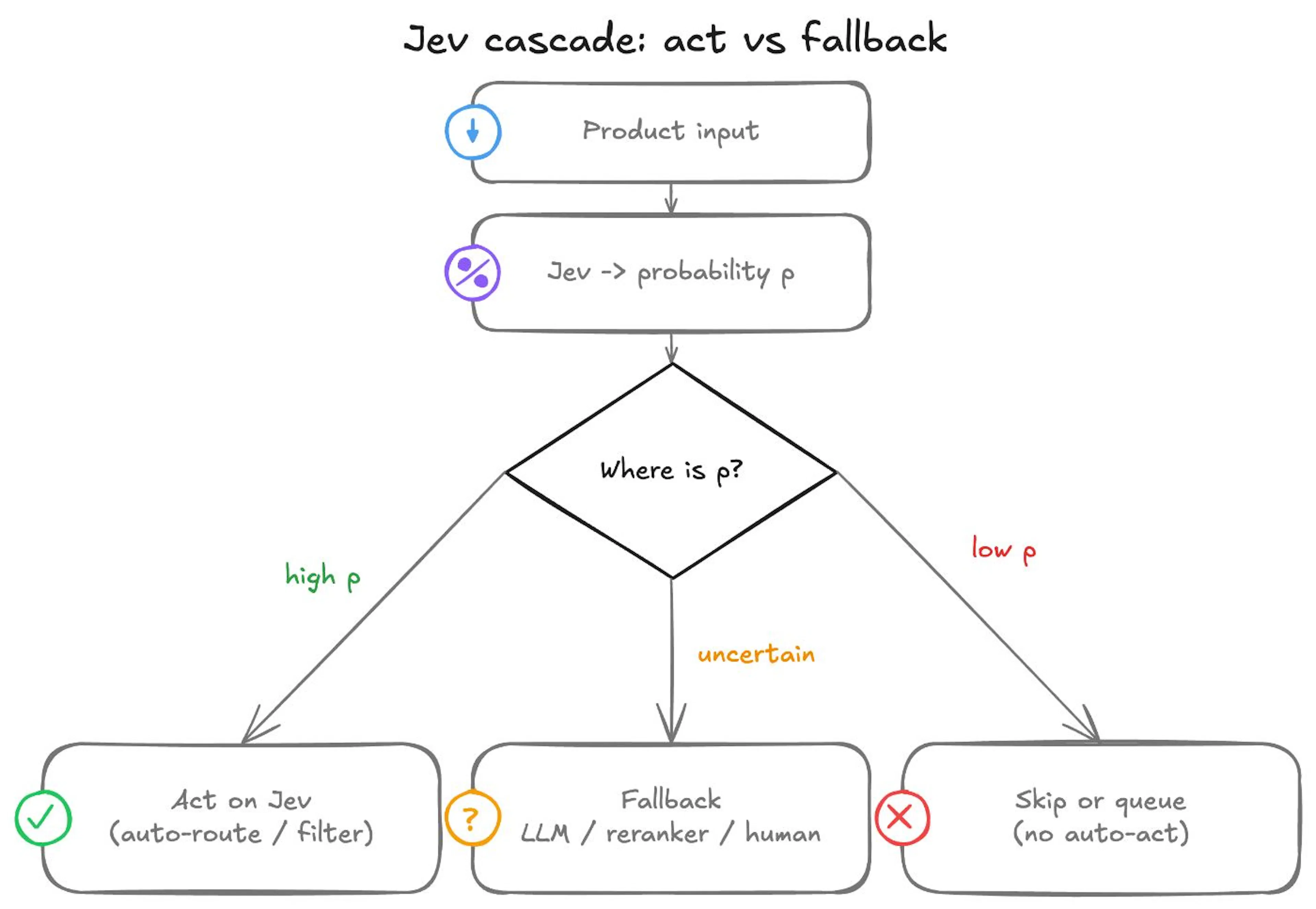 Figure: high p acts automatically; the uncertain band goes to an expensive fallback; low p skips or queues instead of auto-acting.
Product input goes into Jev and comes back as a probability p, and the only interesting question is where that p sits relative to the bands you chose on validation. If p is high -- above the act threshold you picked for this product tradeoff -- you let the feature auto-route, auto-filter, or otherwise act on Jev alone. That is the cheap path, and it is only safe if your eval said high scores are actually trustworthy on your data.
If p lands in the uncertain band, you do not pretend the score is an oracle. You hand the case to something more expensive -- which can be something like an LLM or a human -- because the point of the band is not to look sophisticated; it is to spend latency and dollars only where the fast model is not earning its keep. Same story if p is low -- you usually should not auto-act either, and should escalate the ticket for a person or fall through to whatever default the product already had. A low score is information that the model is not claiming the positive class, and forcing a decision anyway is how you invent false confidence.
Either way, you would ideally measure the full Jev + fallback on the same held-out set you used for Jev-only, or you will not know whether the fallback is fixing the failures that matter.
Closing
Jev is useful because it is fast enough to sit in the hot path and structured enough to call like a function, but it is still a probability model. The community mistake is treating the score like an oracle. The fix is not another framework -- it is basic ML hygiene on your data before the threshold goes to production.
如有侵权请联系:admin#unsafe.sh