Disclosure: I designed and led the build of the system described here as CTO of the company that developed it, and I have a commercial interest in the product. The research write-up is my own work and is available as a preprint (arXiv:2604.03672).

TL;DR We built a classifier that sorts incoming citizen appeals into complaints, applications and proposals, and routes them to the right department. BERT was the most accurate model we tested. We shipped a smaller Word2Vec+LSTM instead. Then load testing showed that neither choice mattered much, because the queue was never in the GPU. It was in the five people doing review.

The job

A government office receives written appeals from citizens. Somebody has to read each one, decide what kind of appeal it is, decide which department owns it, register it, and start the clock, because the response deadline is set by law.

When we measured the existing process, a single appeal took anywhere from 15 minutes for the shortest submissions to 30 for the longest, and operators agreed with the expert-adjudicated label about 67% of the time. That second number surprises people. It should not. Ask trained adults to sort a thousand letters written by angry, tired, formal-sounding strangers into three buckets while the queue keeps growing, and agreement drops fast. Our expert panel reached a Fleiss' kappa of 0.81 (substantial agreement), and they were domain specialists with time to think. The operators, working at speed on live mail, were never going to match that.

So the target was never "replace the operator". The target was "stop making the operator do the boring 80%", in a product that would keep running long after we stopped watching it.

What we tested

Ten thousand real appeals, labelled twice: once by the operators as part of their normal work, then verified and corrected by a panel of three experts. Personal data stripped before anything touched a model. Split 70/15/15, stratified, test set opened exactly once at the end.

Six approaches, in order of how much machinery they need:

The fastText line is the one I keep pointing at. Three minutes of training, no lemmatisation, beats a carefully preprocessed TF-IDF pipeline. Russian has heavy inflectional morphology, so the standard advice is to lemmatise everything before you vectorise. fastText's character n-grams pick up the same regularities on their own and cost you nothing to set up. If you are prototyping on a morphologically rich language and someone tells you to start with a morphology pipeline, run fastText first and see how much of the gap you actually need to close.

Why we shipped the second-best model

BERT won by four points. We put the LSTM in production.

The honest reasons, in order:

1. Hardware. The deployment target was a government data centre with a fixed budget and no GPU inference tier. Two CPU cores and 4 GiB per replica, three replicas.
2. Retraining cadence. We knew we would retrain often on operator-corrected data. Ninety-five minutes versus four hours changes whether retraining is a Tuesday afternoon or a project.
3. Four points of accuracy did not change the workflow. At 78% or at 82%, an operator still reviews the prediction. The output of the model is a pre-filled field, not a decision. Nothing downstream behaves differently.

That third reason is the one that generalises. Before arguing about a few points of accuracy, work out what the marginal point actually buys in the workflow you are shipping into. Sometimes it buys a whole category of automation. Here it bought nothing, because a human was going to look at the screen either way.

I would make the same call again, though I would test a Russian-specific pretrained model first. Multilingual BERT at 82% is well below what the same architecture does on English benchmarks, and part of that gap is almost certainly the multilingual vocabulary rather than the task.

The load test that changed how I think about this

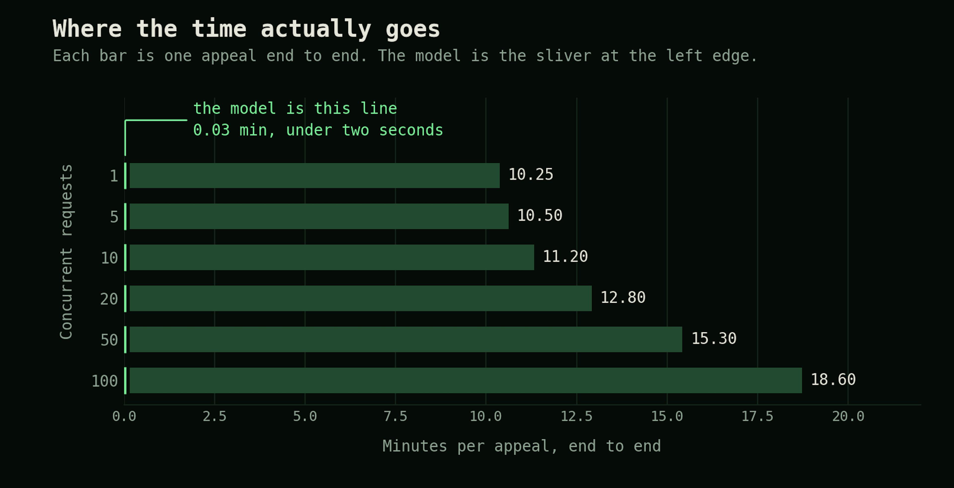
We ran the system under concurrent load and watched processing time per appeal:

Reasonable degradation. At twenty concurrent requests we add about a quarter to our latency. Fine.

Then look at the units. Minutes. Model inference is under two seconds per appeal regardless of text length. Every other second in that column is a human being reading a screen, and the degradation curve is a queue in front of a pool of five reviewers.

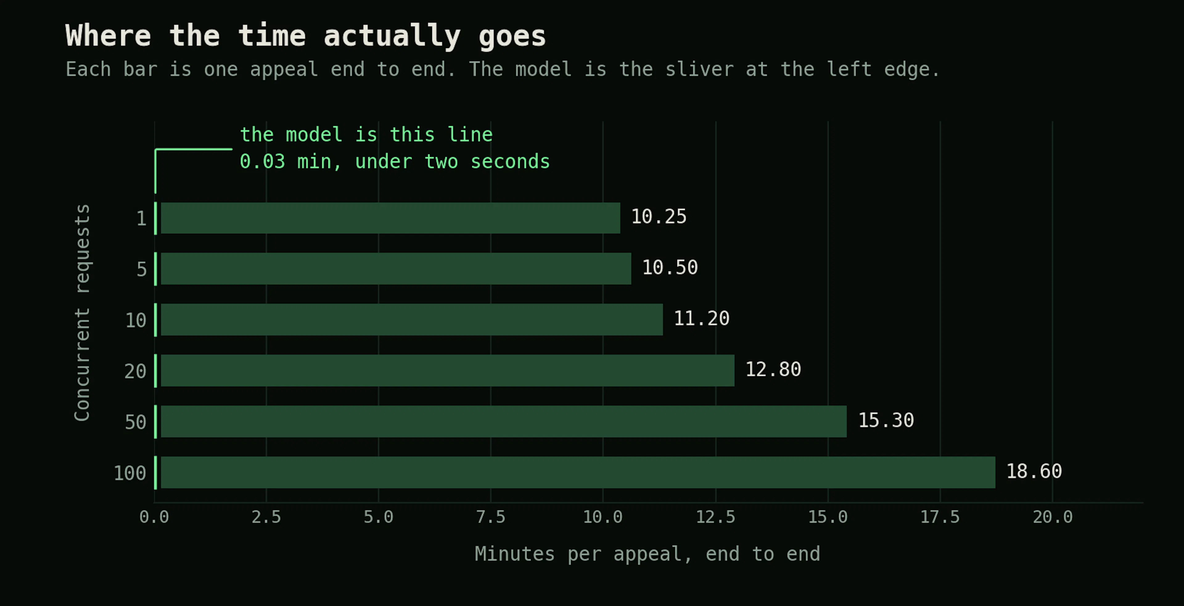
We had built a system where the machine learning component contributes roughly 0.3% of the wall-clock time, and we had spent most of our engineering attention on it. The number that would have moved the product most was not accuracy. It was how many seconds of reading the interface saved the reviewer per appeal, and we had barely instrumented that.

If you are putting a model in front of human reviewers, measure the human step first. It is probably your entire latency budget.

Where the errors actually come from

We pulled a hundred misclassified appeals and read them. Three patterns covered all of them:

• Dual intent, 42% of errors. The citizen complains and requests in the same letter. The elevator has been broken for three weeks, this is unacceptable, please repair it. Is that a complaint or an application? The expert panel argued about these too.
• Bureaucratic register, 31%. The writer has copied a template found online, and the template flattens the intent into standard phrasing that says nothing about what they want.
• Mixed framing, 27%. Factual narration, which reads like an application, wrapped in emotional language, which reads like a complaint.

The first category is not a model failure. It is a taxonomy failure. We forced a single label onto texts that carry two intents, and then measured the model on its ability to guess which one the annotator picked. Nearly half our error budget was a schema decision made before anyone trained anything.

The fix is multi-label output, or a hierarchy with intent as a separate head. That is the main thing I would change about the design, and it is a data modelling decision, not a modelling one.

Human review as an annotation engine

The part that worked better than expected: operators correct predictions as part of their normal job, corrections flow back into the training corpus, and the model gets periodically retrained on them. To find out where that had got us, we exported a sample of production appeals together with the categories the system had assigned, and went through them one by one, marking each as correctly classified or not. More than 95% came back correct, against 78% for the frozen model on the research test set.

The two numbers are measured differently and I would not put them on the same axis. 78% is a model scored once against labels produced independently of it. The 95% is a review of categories that were already on the page, and judging whether a label is defensible is a more forgiving task than picking one from scratch, particularly on the dual-intent appeals that make up most of the error budget. A blind relabel of the same sample would settle that. What the audit does establish is that after several retraining cycles the system was assigning the right category on the large majority of live mail, which is the number that matters once the product is carrying the daily load.

This reframes the review step. On the slide it looks like the unautomated remainder, the thing you are trying to get rid of. In practice it is a labelling pipeline that is already staffed, already funded, and already producing expert-adjudicated data every working day. Budget for capturing those corrections from day one. Log the before and after state of every field an operator touches. It is the cheapest annotation you will ever get.

What I would do differently

• Train embeddings on a proper Russian corpus rather than on ten thousand in-domain appeals. Small corpus, small vocabulary, and the ablation showed 256-dimensional embeddings performing worse than 128, which is what an undertrained embedding space looks like.
• Multi-label classification for intent, per the error analysis.
• Report variance. Every neural result here is a single training run. That is a real weakness, and reviewers are right to press on it.
• Instrument the operator interface as carefully as the model.

Numbers, in one place

78% accuracy on three-class intent, up from 67% manual. A sample audit of production classifications, run after several retraining cycles, found more than 95% correctly classified, with the caveat above about how that was measured. 77% on seven-class routing by topic, ranging from 84% F1 on housing and utilities down to 71% on the miscellaneous bucket, which is exactly the shape you would expect: specialised vocabulary is easy, "other" is not a category. On timing, the automated flow cut end-to-end handling by 53 to 56% in every length band we measured, human review included: 15 minutes down to 7 for the shortest appeals, 30 down to 14 for the longest. Averaged across the four bands that is 54%, from 22.5 minutes to 10.25. That average weights each band equally rather than by how often it occurs in the mail, so the per-band figures are the result to trust. All of these are study-period measurements, taken before the correction loop had been running long enough to matter.

Full method, ablations, confusion matrices and limitations are in the preprint: arXiv:2604.03672.

Vladimir Beskorovainyi is a CTO working on enterprise AI and large-scale data systems. He led the design and delivery of the system described above and wrote its research write-up (arXiv:2604.03672). ORCID 0009-0004-7005-6242.