
The following is a guest post submitted by Matt Larson.The post explains how Matt Larson set u 2026-5-6 04:58:49 Author: www.rtl-sdr.com(查看原文) 阅读量:38 收藏
The following is a guest post submitted by Matt Larson.
The post explains how Matt Larson set up an automated atmospheric wind-sensing station using only locally obtained ADS-B data from an RTL-SDR. Matt's code is available on GitHub.
Listening to the Jet Stream - 100 Days of Wind Sensing with Stock RTL-SDR Hardware
By Matt Larson — Helena Valley Observatory, Helena, Montana
I built a passive atmospheric sensing system using a stock RTL-SDR Blog V4 kit and the included dipole antenna, with no external filtering or amplification.
Over 100 days in Helena, Montana, it logged 5+ million ADS-B messages and produced jet-level wind direction estimates with ~14° mean absolute error versus ERA5 reanalysis on favorable (zonal flow) days — within AMDAR operational reference ranges.
The system requires no aircraft cooperation, no radar, and no onboard meteorological data — only passive reception of ADS-B broadcasts and geometric analysis of reciprocal flight tracks.
This turns an RTL-SDR from a visualization tool into a measurement instrument. Instead of asking "what aircraft are overhead," you can ask "what is the atmosphere doing above me right now?"
The Bet
It started as a $50 bet with myself.
I had no formal background in atmospheric science. No lab, no funding, no institution behind me. Just a house built in 1894 in Helena, Montana, a Linux box, and a question I couldn't stop thinking about: could you use the aircraft already flying overhead as atmospheric sensors — without touching them, without their cooperation, without anything except listening?
The worst case was a $30 receiver and some wasted evenings. The best case was something I couldn't quite articulate yet.
I plugged in an RTL-SDR Blog V4 kit I bought on eBay, pointed the small dipole antenna that came in the kit at the sky, and started asking questions.
That was January 17th, 2026. One hundred days later, I'm writing this with a longitudinal archive of more than 5 million records, validated jet-level wind estimates within the AMDAR operational accuracy range, a documented terrain channeling signature for the Helena Valley, and a surface-level signal consistent with the timing and structure of the January-February 2026 Sudden Stratospheric Warming event, validated against ERA5 and radiosonde data but not independently attributable.
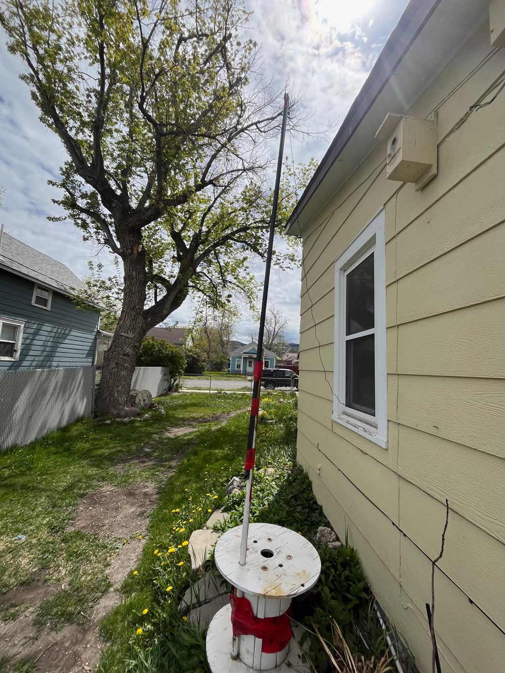
No dedicated 1090MHz antenna. No external filter. No fancy mast. The stock dipole that came in the kit, tuned to 1090MHz.
This is what I learned. And at the end I'll tell you exactly how to start.
What You're Actually Doing
When an aircraft equipped with ADS-B transponds, it broadcasts its GPS position, altitude, groundspeed, heading, and a timestamp. Your RTL-SDR receives that broadcast passively — you're just listening. No radar, no active emissions, no interaction with the aircraft at all.
Most people use this to watch planes on a map. That's genuinely fun. But there's more in that signal than position data.
An aircraft's groundspeed is its speed relative to the ground. Its airspeed is its speed through the air. The difference between those two numbers — the vector difference, accounting for direction — is the wind. The aircraft doesn't measure wind directly, but the relationship between what it's doing through the air and what it's doing over the ground encodes the wind field it's flying through.
The problem is that ADS-B gives you groundspeed, not airspeed. So how do you recover the wind?
The answer is geometry.
If two aircraft fly the same route in opposite directions, one sees a tailwind and one sees a headwind. The difference in their groundspeeds is twice the wind component along that axis. Divide by two, and you recover the wind — without ever measuring airspeed.
No airspeed required. No heading required. Just groundspeed and geometry.
That's the foundation of what I built: a passive atmospheric sensing station that extracts wind information from aircraft that are already flying over my valley every day whether I'm watching or not.
One important note on aircraft types: heavy jets and regional aircraft have different typical true airspeed values at the same altitude. The solver accounts for aircraft class when making TAS assumptions, and estimates are validated against external reanalysis data rather than treated as precise measurements in isolation.
The Observatory
The hardware is simple.
RTL-SDR Blog V4 kit from eBay. The small dipole that comes in the kit. Tuned to 1090MHz. A Linux machine running Arch. readsb decoding the signal. A Python pipeline I wrote from scratch to archive, segment, and analyze the data.
That's the whole stack. No proprietary software. No cloud dependencies. No subscription. Everything runs locally and everything is mine.
The software architecture has three layers.
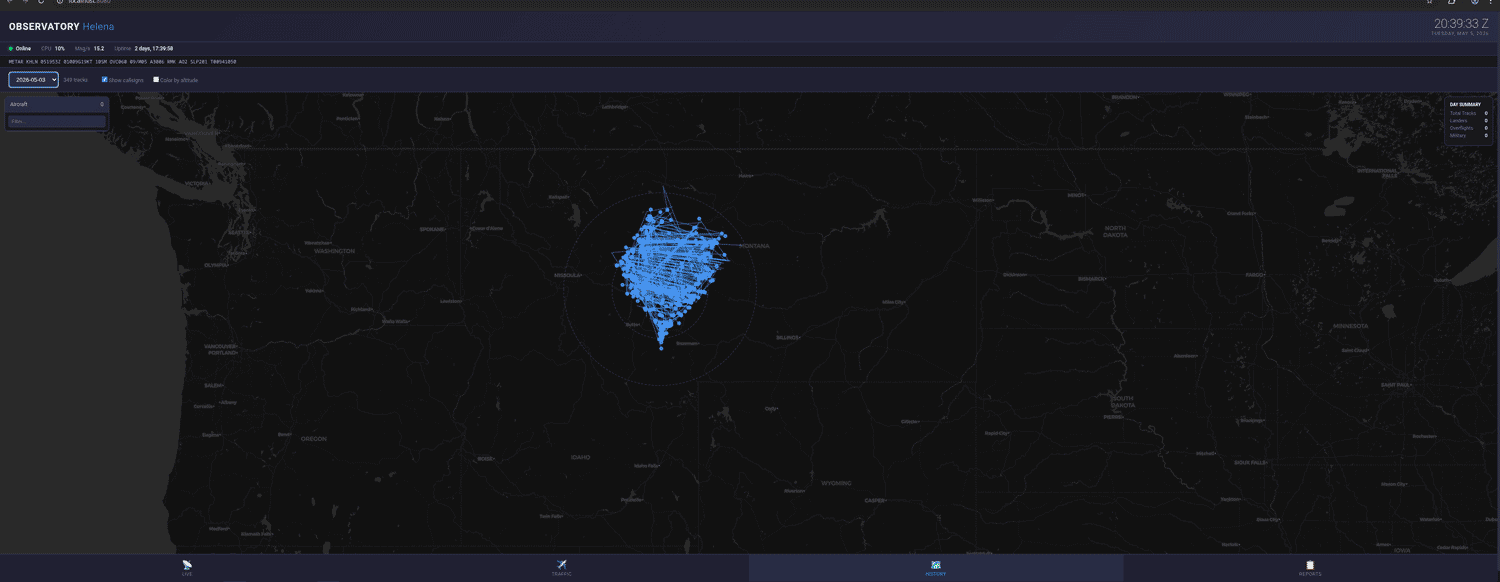
The first is the archive. Every observation logged to JSONL files — position, altitude, groundspeed, callsign, registration, timestamp — every five seconds, continuously, without gaps. After 100 days that archive contains more than 5 million records representing roughly 300 unique aircraft per day.
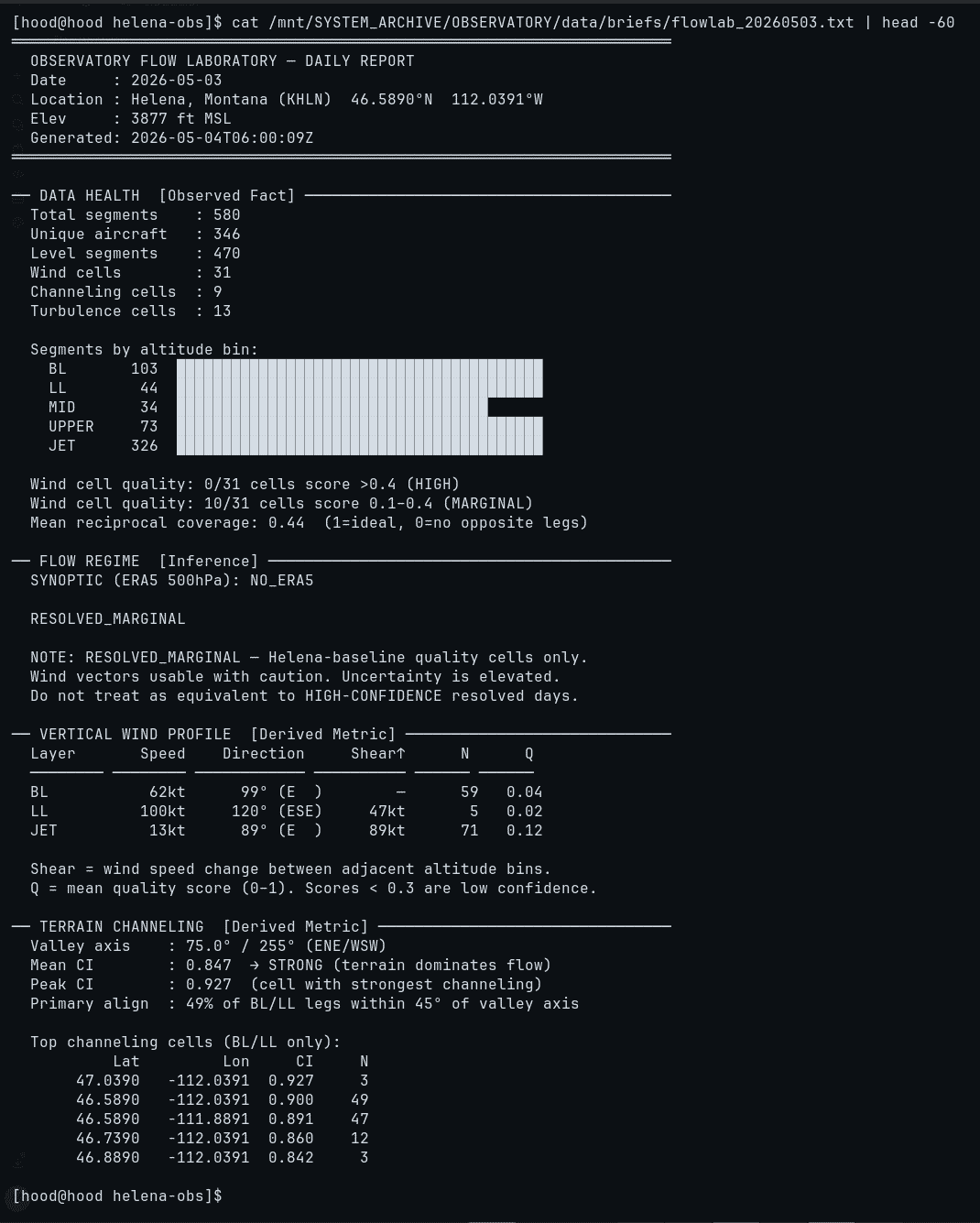
The second is the Flow Lab. The atmospheric analysis pipeline. It runs four stages each night: segmentation breaks continuous aircraft tracks into straight-line level-flight segments; wind solving applies the reciprocal pair geometry to extract wind vectors per altitude layer; terrain analysis measures how strongly the valley's topography constrains aircraft tracks; and reporting produces a daily brief in plain text that I read the next morning like a weather report from my own kitchen.
The third is the Signal Lab. RF characterization — near-field and far-field RSSI variance, anomalous propagation events, terrain shadow mapping, free-space path loss residuals. The radio environment of the Helena Valley, documented day by day.
Everything automated. Everything archived. Every output reproducible from the raw JSONL files.
What the Methodology Requires — And What It Doesn't
I want to be honest about what this system can and cannot do before I tell you what it found, because the limitations matter as much as the results.
The reciprocal pair wind solver works under specific conditions. It needs enough aircraft flying opposing tracks at similar times and similar altitudes. On busy traffic days with good reciprocal coverage it produces clean wind estimates. On quiet days or days with limited crossing geometry it produces nothing — and says so explicitly rather than guessing.
Wind direction is recoverable with reasonable accuracy under these conditions. Wind speed carries inherent uncertainty because the solver depends on assumptions about aircraft true airspeed. Speed estimates are reported with explicit uncertainty bands and are not treated as precise measurements.
The system fails gracefully on trough days — when the jet stream is curved and the flow is complex. On those days the solver flags the output as UNRESOLVED and produces no wind estimate rather than a wrong one. Knowing when you cannot measure something is part of measuring it honestly.
Every output in the daily brief carries a label: OBSERVED FACT, DERIVED METRIC, or INFERENCE. Nothing gets promoted to a finding without meeting explicit quality gates. The methodology is documented in enough detail that anyone could replicate it and get comparable results.
What 100 Days Found
Jet-level wind direction.
The reciprocal pair solver produces daily wind direction estimates at five altitude layers. At the jet stream layer — above 36,000 feet — the day-to-day directional consistency across the archive shows a correlation of R=0.954. That's a strong unimodal signal. The jet over Helena runs westerly the vast majority of days, with documented exceptions on trough and transition days.
On days with zonal flow — when the atmosphere is well-organized and the jet is running straight — I compared estimates against ERA5 reanalysis data from the Copernicus Climate Data Store. Here are the actual numbers:
| Metric | Value |
|---|---|
| ZONAL days with ERA5 comparison | N=21 |
| Mean angular error (MAE) | 14.3° |
| Median angular error | 13.5° |
| Best day | 0.3° error |
| Worst day | 38.3° error |
| Days with STABLE solution (robust to parameter changes) | 68 of 81 (84%) |
| Day-to-day jet direction consistency (R) | 0.954 |
| AMDAR operational target range | 10–20° |
A $30 kit with a stock dipole antenna on a rooftop in Montana is producing estimates that land inside the AMDAR operational accuracy range on favorable days. On trough days the system fails and says so. That's also a result.
Terrain channeling.
The Helena Valley runs roughly ENE/WSW — 75 degrees and 255 degrees. The terrain channeling index measures what fraction of low-altitude aircraft tracks align within 45 degrees of that axis.
The mean channeling index across 100 days is 0.855.
To put that plainly: the valley's terrain is so effective at constraining low-level airflow that it dominates aircraft track orientation regardless of what the synoptic weather pattern is doing that day. Aircraft aren't intentionally following the valley — their routes are set by ATC. But the wind field the terrain creates pushes their ground tracks toward the valley axis. The terrain writes its signature into the aviation data every single day, zonal or trough, January or May.
That signal is geographically structured. The channeling index is strongest in the valley core — CI above 0.90 near the center of the Prickly Pear Valley. It weakens at the eastern exits where the terrain opens toward the Missouri River drainage and the Elkhorn foothills. The valley acts like a funnel: strong forcing at the narrow western end, diminishing constraint as the terrain opens to the east. The passive observer mapped that transition without anyone telling it where to look.
Atmospheric events.
The 100-day archive contains 43 documented atmospheric events: 21 split-column events where the boundary layer and upper atmosphere were moving in opposite directions, 11 shear events with elevated mid-level turbulence signatures, 3 probable mid-level shear zones independently verified against IGRA2 radiosonde data, and 2 rough days with elevated boundary layer turbulence indices.
The March 8th event is the clearest example. The system flagged elevated turbulence at both the boundary layer and mid level simultaneously — boundary layer kinematic turbulence index 12.1 knots, mid level index 19.6 knots. IGRA2 radiosonde data confirmed a low-level jet developing through the day with 52 degrees of directional shear within the boundary layer and speed shear at the boundary layer to mid level interface. The passive observer detected the event. Independent radiosonde data confirmed the mechanism.
A surface signal consistent with the Sudden Stratospheric Warming.
In early February 2026 a major Sudden Stratospheric Warming event occurred — the polar vortex split into two lobes around February 15th, confirmed by NOAA and multiple meteorological agencies. The observatory was running continuously through this entire period.
The archive shows what happened from the ground up. In late January the jet stream over Helena was running at an estimated 88 knots westerly — consistent with the pre-SSW pattern. In mid-February the system flagged a dramatic collapse: a 73% drop in the jet proxy falling to roughly 24 knots. February 18th through 22nd showed persistent Signal Lab anomalies with anomalous propagation events clustering to the SSE. February 23rd through 25th produced two PROBABLE mid-level turbulence events verified by radiosonde — mid-level shear zones consistent with a disorganized recovering jet. February 24th was the archive's strongest validated day: four independent internal proxies converging on a jet estimate of 139 knots, confirmed against ERA5 data.
To be precise about what this means: the observatory measures aircraft groundspeed residuals — it does not measure the stratosphere directly. The archive cannot independently confirm the SSW as the cause. What it can confirm is that a surface-level signal consistent with the timing and structure of a major SSW was real, measurable, and validated against ERA5 and radiosonde data. The passive observer caught it. The independent data confirmed the structure.
A $30 kit with a stock dipole, in a kitchen, in Helena Montana.
What Happened When I Went Outside
At about day 60 I started showing the work to people.
I walked into a flight school near KHLN airport. Introduced myself, explained what I'd been building. The owner sat with me for 45 minutes. He gave me an aviation weather handbook. That conversation — a working pilot engaging seriously with what a passive ground station was measuring — told me the methodology was asking the right questions even if I didn't have all the answers yet.
I sent a cold email to an atmospheric scientist. Dr. de Haan — who I later discovered is considered the godfather of this type of science — was working in a similar space but with a more direct approach. His methodology reads meteorological data from Mode-S transponder messages directly. Mine derives it from geometry. I found out he existed after I'd already built my own approach from scratch, which was a relief — it meant I wasn't crazy, just doing it the hard way. He replied that he would review the methodology. I'm still waiting. That's honest. The door is open.
Then something unexpected happened. In a Facebook group where I'd been sharing the work, a United States Air Force F-16 pilot read what I was doing and reached out. He had one question and two comments about the wind estimation methodology — questioning the TAS assumption across aircraft types, pushing back on the turbulence classification, and suggesting vertical velocity indicators as a potentially cleaner turbulence signal than groundspeed.
He wasn't wrong on any of it. The methodology got better.
An F-16 pilot giving aerodynamic feedback to a guy with a stock dipole antenna and a Linux box in Helena Montana. Under 90 days in.
I'm telling you this not to impress but because it matters for what the approach can become. These are people who would recognize if the methodology was nonsense. They engaged because the work was honest. The outputs were constrained within what the data could actually support. The failure modes were documented. The limitations were stated.
Honest work finds its audience.
The Bigger Picture
I want to say something carefully about what this could mean beyond my valley.
The Helena Valley Observatory is one station. One fixed location. One passive receiver. Its findings describe the atmosphere above a specific valley at a specific elevation between specific mountain ranges. They do not generalize without replication.
But the methodology generalizes. Anywhere aircraft fly, the reciprocal pair geometry works. The Flow Lab pipeline is documented and reproducible. The hardware is a $30 kit with a stock antenna and a Linux machine.
There are regions of the world with almost no upper-air atmospheric data — no radiosondes, no AMDAR coverage, no radar. Some of those regions have commercial aviation flying overhead every day. The aircraft are already doing the work. Someone just needs to listen.
I'm not claiming the Helena system is ready for operational use. The methodology needs more validation, more external review, more replication at other sites. The failure modes need to be fully characterized before anyone trusts the outputs for anything beyond research.
But the proof of concept exists. One person, one 1894 house, one $30 kit with a stock dipole antenna, and 100 days of honest science. Wind estimates inside the AMDAR accuracy range. A terrain channeling signature consistent with the physical geography. A surface signal consistent with a major stratospheric event, confirmed by independent data.
The floor of what's possible with this approach is higher than I expected when I made the bet.
How to Start
Minimum setup:
- RTL-SDR Blog V4 kit
- Stock dipole antenna (tuned to 1090MHz)
- readsb for decoding
- JSON logging at 5-second intervals
- A Linux machine with ~50MB/day storage
30-day baseline:
- 200–300 aircraft per day depending on your location
- Reciprocal track pairs accumulate naturally with traffic
- Wind inference becomes possible on high-traffic days
- Don't build the analysis pipeline yet — let the archive grow first
Validation (don't skip this):
- ERA5 reanalysis — freely available from the Copernicus Climate Data Store
- IGRA2 radiosonde data — nearest upper-air station to your location
- The data has to be accountable to something outside itself
The honest timeline:
The methodology I built took 100 days to stabilize. The first version of the wind solver produced plausible-looking results that turned out to be wrong in ways I couldn't detect without external validation. ERA5 and IGRA2 cross-checking revealed failure modes I didn't know existed. The system got better by failing honestly and documenting the failures.
Every location is different. Every valley has different terrain, different traffic patterns, different failure modes. The Helena findings don't transfer to your site without your own 100 days.
Start simple. Log everything. Stay honest about what you know and what you don't. Let the archive earn its findings.
The aircraft are already up there. They've been flying over your house for decades. All you're doing is listening.
Code available at https://github.com/HelenaValleyObservatory/helena-valley-observatory
Acknowledgments
Carl Laufer and the RTL-SDR.com community — for building hardware worth building with, and for creating a platform where people share what they learn.
The atmospheric science community for making ERA5 and IGRA2 data publicly available. Cross-validation against real data is what separates science from wishful thinking.
Dr. de Haan for being willing to look at the work. The flight school owner in Helena who gave me the Aviation Weather handbook and 45 minutes of honest conversation. The F-16 pilot who read what I was doing in a Facebook group and sent feedback that made the methodology better.
And the aircraft. The thousands of pilots who fly over the Helena Valley every day without knowing someone in a 132-year-old house is listening.
Matt Larson
Helena Valley Observatory
Helena, Montana
May 2026
The observatory runs on curiosity, Linux, and a $30 bet that turned out to be worth taking.
如有侵权请联系:admin#unsafe.sh