This blog post is part of a recent personal investigation into a malware loader known as Coper. Rather than providing a full, line-by-line dissection of the malware, the goal is to introduce a high-level approach to triaging an Android native library.

An increasing number of Android malware families now rely on native libraries to hide their payloads, making reverse engineering a little bit more challenging. Nowadays, having an understanding of what is happening on native libraries is a fundamental skill that needs to be mastered, since it also represents a pivotal point to start investigating other malware families and even architecture.

💡 Through this blogpost, I try to make it as more understandable as possible, making reverse native libraries a little bit less disorienting. Because of that, I would like to make a soft introduction to native libraries, going against a real world example, covering something that goes over the mere basics, without losing the actual focus on learning new things along the way.

Reference: 1e38419cea3379d8992d165f842f3fd78e9da32aa7f04bcb19e3bdf71d109e2f

From Java to Native Code Connection

To execute a function from a native library, the Java code must first declare a corresponding native method. When this Java-declared native method is invoked, the paired native function within the compiled library (ELF/.so) is executed.

In Java, a native method looks like a regular method declaration, with two key differences: it is marked with the native keyword, and it contains no implementation. This is because the method’s logic resides entirely in the compiled native library rather than in Java code.

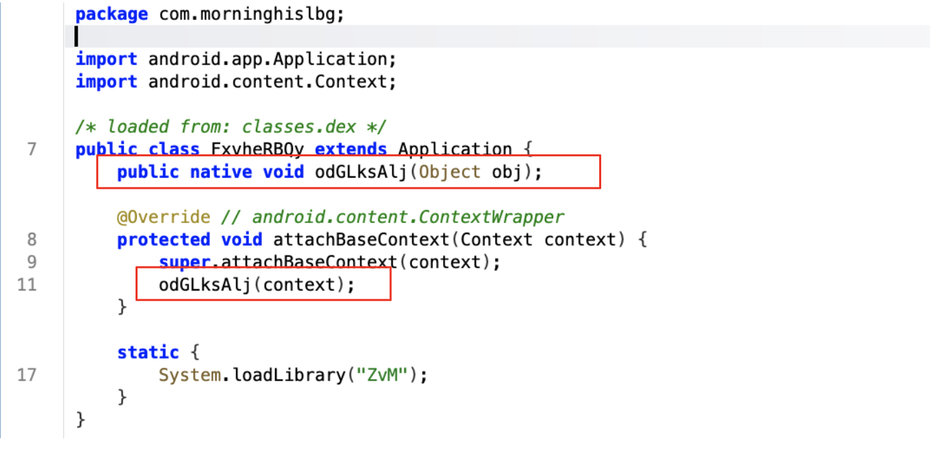
Figure 1: Loading Native Library

The bytecode in an Android application’s .dex file declares the native methods. Each of these declarations is paired with a corresponding subroutine in a shared native library. Before any native method can be invoked from Java, the application must load the shared library (.so file) using System.loadLibrary or System.load. When one of these loading methods is called, the JNI_OnLoad() function in the shared library (if present) is automatically executed.

💡 If you start exploring the native library straight way, you will see that we do not have the On_Load function. This could happen for many reasons. JNI_Onload method usually runs immediately when the library is loaded, breaking this pattern could give some advantages to attackers that could use a dedicated method instead of relying on the builtin routine, having full control over the library running methods under specific conditions (e.g., after verifying device environment variables to detect root or emulation). Moreover in this way its also possible to bypass automation techniques that look for common and standard routines.

In order to run a native method from Java, the native method must be ‘registered’, meaning that the JNI knows how to pair the Java method definition with the correct function in the native library. This can be done either by leveraging the RegisterNatives JNI (static linking) function or through discovery based on the function names and function signatures matching (dynamic linking) in both Java and the .so . For either method, a string of the Java method name is required for the JNI to know which native function to call.

In this example we are going to see the usage of function name and signature discovery. In order to pair the Java declared native method and the function in the native library the naming conventions need to meet specific requirements. A native method name needs to be concatenated with the following components:

• the prefix Java_
• a mangled fully-qualified class name
• an underscore (“_”) separator
• a mangled method name

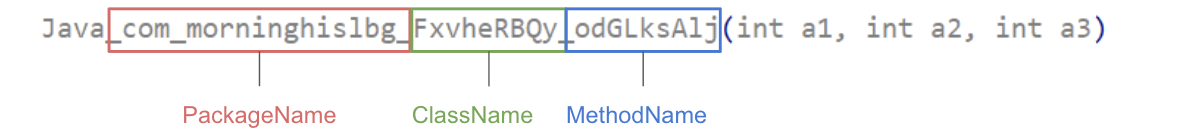
Figure 2: JNI function signature

Looking at the signature, it’s clear that something odd is still there. There are three int parameters that we have not identified in the Java call. What are they? Those parameters are part of the calling convention that actually hides a few things that our disassembler missed. If you look at JNI documentations its possible to rewrite parameters as follow:

void Java_com_morninghislbg_FxvheRBQy_odGLksAlj(
    JNIEnv *env,
    jobject this,
    jobject context
)

• JNIEnv *env represents a getaway to the entire Java world. If we need to call Java methods, classes, objects, access or instantiate strings, etc… It could be basically seen as a pointer to a structure that contains JNI interface function pointers.
• jobject this is the Java object instance the methods belong to. This object allows the C function to access instance variables of the Java object itself, giving also a chance to call other methods on the same object
• jobject context is the actual parameter passed from Java

💡 I know, all the information provided so far could be a little bit disorienting, however, before proceeding directly examining the native code, it’s important to get some preliminary information about JNI specification and functions and include them within your decompiler/disassemble tool, missing this step would literally make the reverse session a nightmare since your are not able to distinguish native methods and classes that will be used to follow the overall flow. You can import those files directly in IDA or Ghidra.

Resolving Names and Creating Structure

Exploring the code through a disassembler and guided by the previous insight we could easily go directly to Java_com_morninghislbg_FxvheRBQy_odGLksAlj function. However, as soon as we open up the code, we are flooded by a quite long list of variables and some strings as well as a lot of strange code that appears to be called from an offset related to the first parameter.

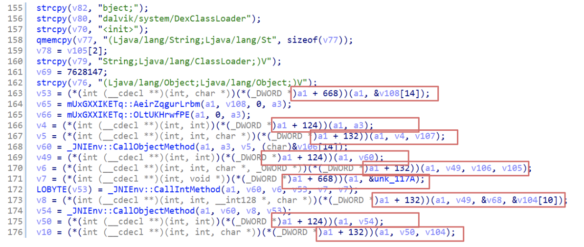
Figure 3: Unresolved JNI names

To make the code more readable, its time to set parameters properly, according to the one identified in the previous section. In this case a1 its the JNIEnv * , so we could expect properly resolved functions.

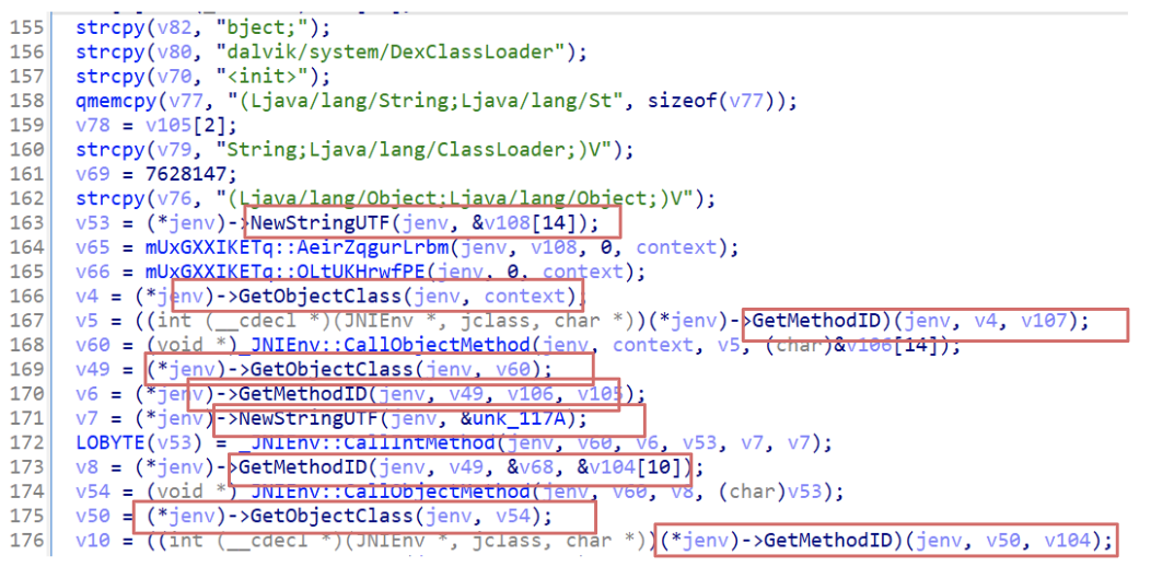
Figure 4: JNIEnv type structure set

Resolving type and renaming the variables properly we could have a little bit more readable code, however, it’s far away from being explorable to reverse and understanding the general workflow. If we look at the beginning of this function we could easily spot a long sequence of strcpy with some interesting values like: com.morninghislbg:raw/urdvipkyjahgh and getResources. Those are quite interesting since we are seeing a potential resource and a method to retrieve that. Why? Moreover, we are also able to see some strings related to reflection techniques such as: dalvik/system/DexClassLoader, setAccessible or even Reflect/Field.

From here, its possible to make hypothesis and exploring few questions:

• What is that resource in the APK files?
  • Are those resources packed or encrypted? Does it contain code? Why is it used? Is there any relation between that and the DexClassLoader method?

From here there are a couple of options, resolving names for all variables (or at least most of them) or start exploring our hypothesis hoping for the good.

💡 Generally speaking, renaming variables is one of the most important tasks before doing anything else. From this point, you could take your time starting renaming variables, setting proper types and structure until you will have a clear idea of what is happening. A good trick that I use most of the time is to start renaming variables that are involved in function calls and then let me drive from hypotheses that could also arise from resolved names. There aro no good or bad options, usually it depends also from the time you have for analyzing a sample.

Because this is a kind of introduction to this topic, it’s better to explore the code closely using a more structured approach. First of all, let’s start from the very beginning where the strcpy functions are invoked. From there we could be able to see a few patterns that should be a hint about how information is stored also in the original program.

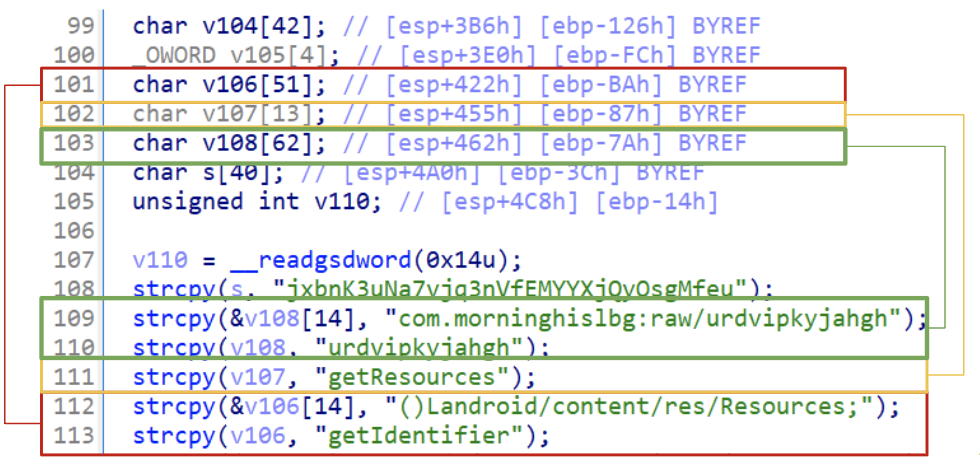
Figure 5: Sequence of resolved strings

If your code looks like the figure above, it is caused by the obfuscation in place. Strings are stored on stack, however, the disassembler did not fully understand the whole structure and did its best to retrieve strings giving to us a partial, but still a good result. An example is the v108 where there is an array of 62 chars that contains two strings one after another. A more readable code should look like the following:

  strcpy(&v108.fullpath_resource, "com.morninghislbg:raw/urdvipkyjahgh");
  strcpy(&v108.resource_name, "urdvipkyjahgh");

In order to make the overall code more there are two ways, using a global structure that embed this information or renaming variables directly as they are trying to include information about their values.

💡 Since I’m trying to make some references that go over the mere Coper analysis, I will go through the structure path. However, it’s important to keep in mind that creating a structure does not represent the best approach in general, it’s all about time and purpose. From time to time, I go straight to the point of renaming very few variables, especially if the malware is already known and documented.

In order to start creating a global structure that will contain all those variables we should inspect the code a little bit more. If we see the strcpy we could spot the offset where the first variable is written.

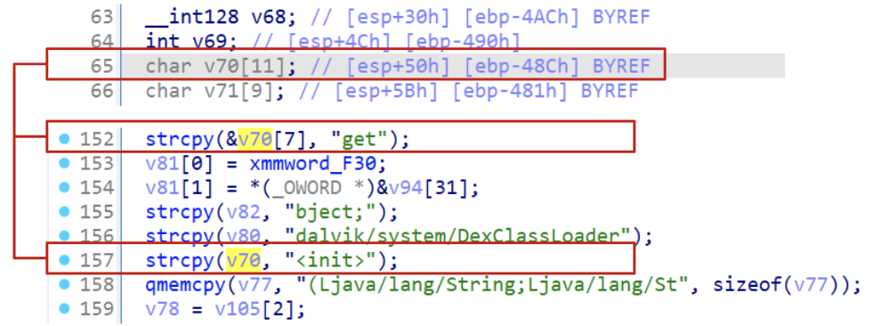
Figure 6: ESP identification for calculating malware configuration structure

From the figure above it is possible to see that the very first variable is located at esp+50h, then exploring the stack all the way up it is possible to see that the latest variable is stored at esp+4C8h. If we calculated the size from those two values its possible to see that our struct should be 0x47C bytes.

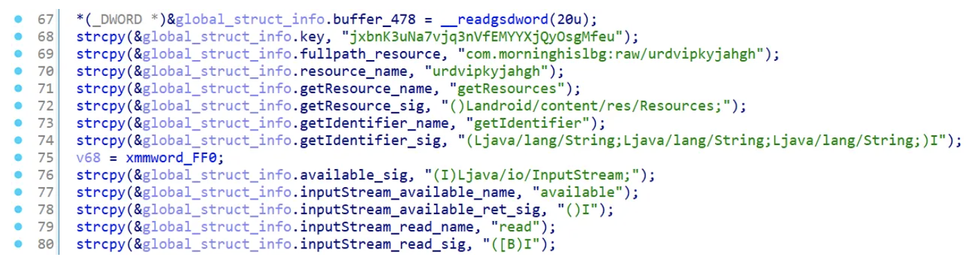
Figure 7: Malware structure applied and variable renaming

Function Triage

Now that we have resolved most of the names importing JNI functions and renaming variables through a proper structure, everything should be more readable and easier to get understood. This function could be divided into three main parts.

• Collecting resource information to see if the encrypted payload is available

  

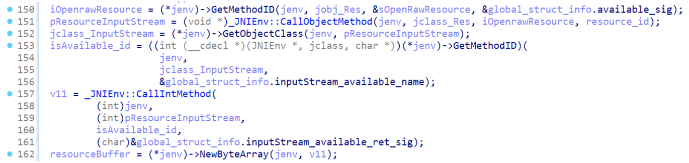
  Figure 8: Check for encrypted payload

• Allocating a buffer, according to the resource size, that is going to contain the encrypted data

  

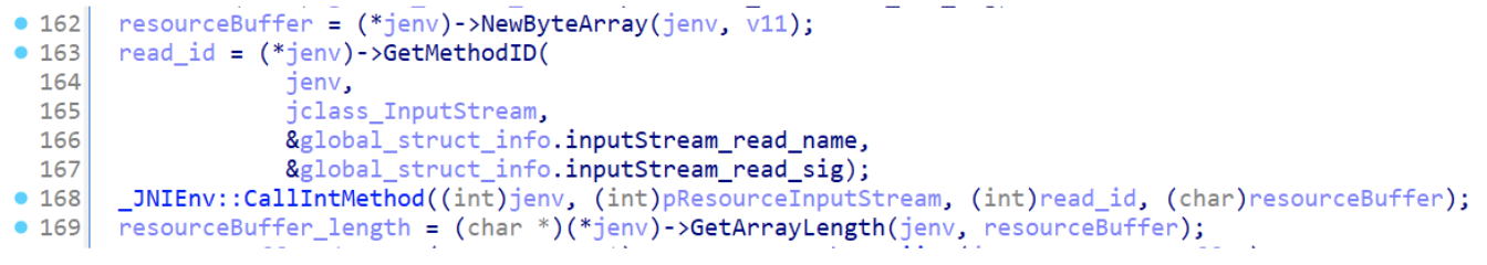
  Figure 9: Allocate memory for decrypted buffer

• Decrypt the resource, verifying that the process has been completed correctly and in the end load the .dex file into the application context.

  

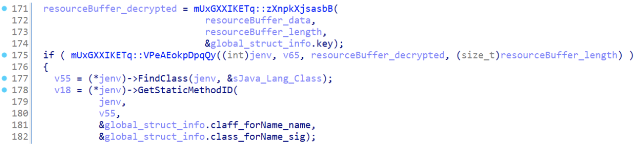
  Figure 10: Payload decryption function

💡 As expected the general flow of this library is pretty straightforward once you rename variables according to JNI specifications and strcpy values. Most of the effort in this case has been taken by the renaming task. I know, it could be boring and tedious but it happens most of the time that “complex” code just lacks proper renaming to get understood.

However, even if the general flow appears to be quite straightforward, how was it possible to understand that a decryption routine was in place? And which algorithm has been used?

Payload Decryption

When exploring code, especially cryptographic routines, start looking for known patterns that usually give great hints about the algorithm itself and most of the time point towards the right solution. From the information collected we could easily start exploring zXnpkXjsasbB that takes key, buffer and the buffer_size.

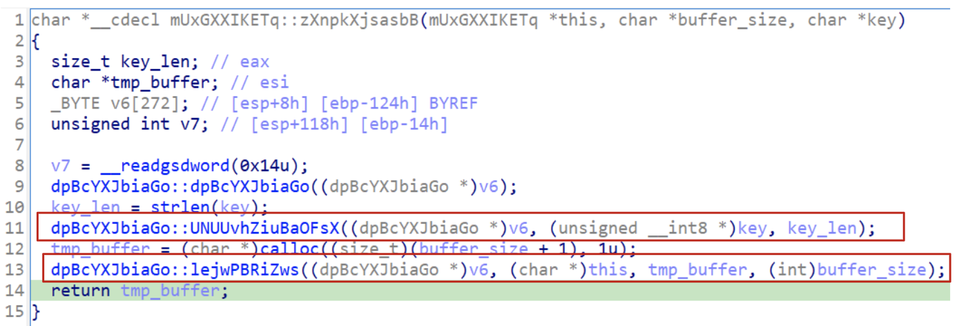
Figure 11: Identification of cryptographic functions

From here there are two main functions to explore ( it’s worth noting that dpBcYXJbiaGo doesn’t affect decryption).

Exploring the UNUUvhZiuBaOFsX function we could immediately spot interesting values. It starts initializing a few variables using a structure.

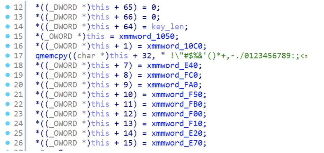
Figure 12: RC4 S-Box initialization

However, what do those xmmword_ values contain? Looking at the first two values we see some interesting values that go from 0 to 31. Exploring all those values we could discover that its actually goes from 0 to 255. Does it ring any bells?

Figure 13: RC4 S-Box example

If not, we could start exploring a little bit more the rest of this function. Let’s get some insight from what we see without renaming anything.

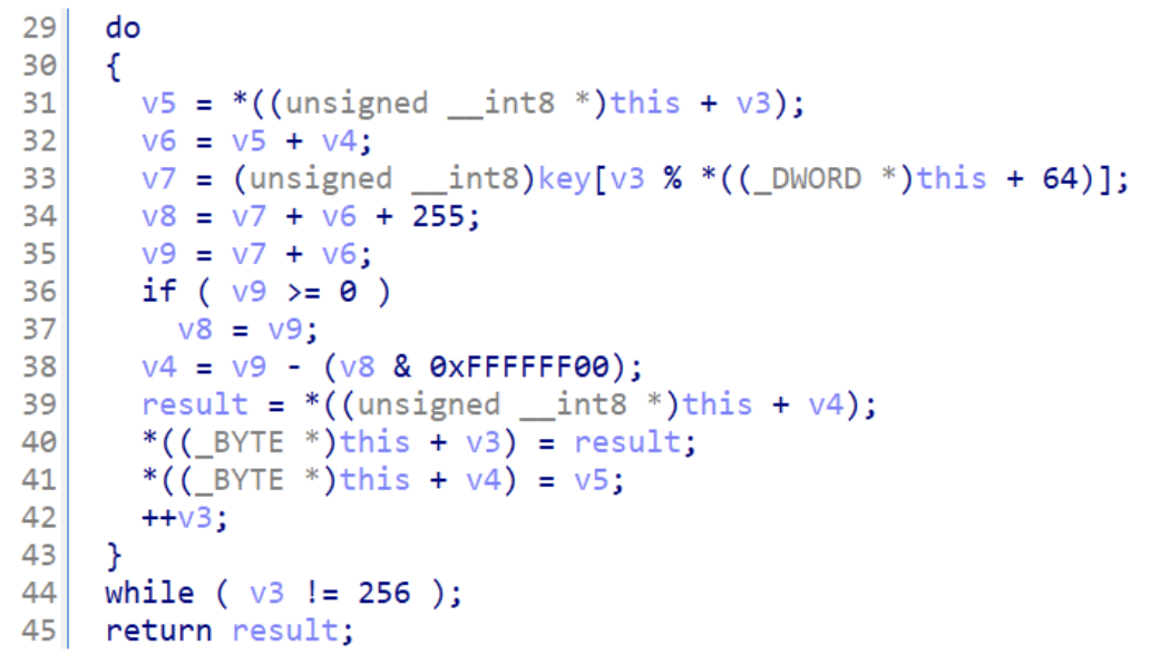
Figure 14: RC4 KSA

• line 33: key[i % key_len]
• line 34 - 38: (value) % 256
• line 39-41: swap(S[i], S[j])

All those steps are done 256 times. What is happening in this code? Well, trying to use some known patterns from cryptographic functions, this is a good indicator that we a re dealing with RC4 key scheduling phase that could be seen (without obfuscation) through those few lines of pseudocode:

j = 0
   for i = 0 to 255:
       j = (j + S[i] + key[i mod keylen]) mod 256
       swap(S[i], S[j])

So we could rename this function as rc4_ksa. As expected, since the algorithm is divided in two parts, the next function is the PRGA (Pseudo-Random number Generation Algorithm) that is going to include also the XOR operation with the encrypted resource bytes.

Now that has been possible to identify the RC4 routine, let’s try to understand the PRGA using the reverse strategy, starting from a pseudocode and trying to conciliate it with what we have in our disassembler. A general version for the prga, should looks like similar to this:

for each byte in buffer:
    i = (i + 1) % 256
    j = (j + S[i]) % 256
    swap(S[i], S[j])
    K = S[(S[i] + S[j]) % 256]
    plaintext = K XOR ciphertext

Once we open up the lejwPBRiZws function, we should be able to spot some pattern that was already seen in the previous function. Basically, the modulo is hidden through add , & operations that tries to make this code a little bit less understandable. However, since this pattern has been already resolved, we could safely mark it and skip to the next block of instructions that are the XOR routine that decrypts the actual payload (blue rectangle).

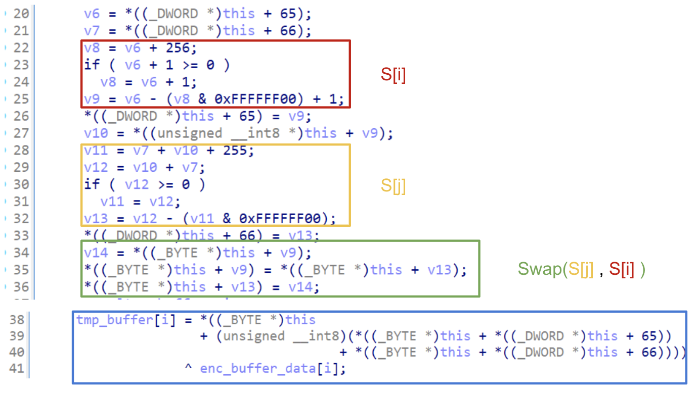
Figure 15: RC4 PRGA and XOR

💡 At this point, I hope that everything sounds a little bit more clear. Obfuscation is something that prevents the code be seen clearly, but once you unfold the the most importants variables everything starts to make sense. There is no perfect solution, the idea is always start making hypothesis and continuously challenging them.

Automation

As always, making some automation about the overall process is also part of the fun. Because of that, I tried to make a script that takes care of all those steps decrypted in this blogpost.

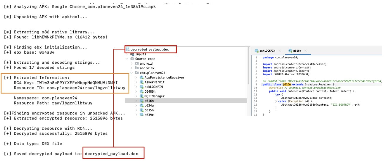
Figure 16: Decrypted payload

💡 It’s worth mentioning that the script provided has some limitations related to the target architecture (x86), moreover, it sometimes breaks because of APK malformation in place. Because of that, modifying the script directly doesn’t help us. To handle those errors correctly, you should create a pipeline that cleans up the APK in order to be properly processed by decryption and/or configuration extraction tools. Nevertheless, a more structured approach including dynamic analysis is actually encouraged, because of potential complexity that could arise exploring different builds.

Conclusion

This blog post aims to provide a soft introduction to Android native libraries and how to investigate them to extract useful information that can be reused in further analyses, as well as to develop effective decryption or unpacking routines. For a real-world example, the Coper loader was chosen due to its widespread presence and slightly more advanced logic, which includes a degree of obfuscation. Generally speaking, reversing Android native libraries can sometimes feel disorienting, especially without prior experience in x86 or ARM binaries. However, with the right mindset and some patience, it becomes feasible. Most of the techniques demonstrated in this blog post are broadly applicable: renaming variables, recognizing common code patterns, forming hypotheses, and testing them are always valid approaches, regardless of the specific malware being analyzed.

Hope you had fun and really enjoyed this blogpost. Thank you for reading! :)

References:

RC4 algorithm specifications:

• TALOS blog
• GoggleHeadedHacker (I really love this blog, it’s my favourite reference for a lot of topics)

JNI references

• Oracle JNI function reference
• Oracle JNI type sgnature

Sample:

• Coper Loader

Coper Unpacker/Decryption script:

• coper_unpacker.py