Currently, Cloudflare Radar curates a list of observed Internet disruptions (which may include partial or complete outages) in the Outage Center. These disruptions are recorded whenever we have sufficient context to correlate with an observed drop in traffic, found by checking status updates and related communications from ISPs, or finding news reports related to cable cuts, government orders, power outages, or natural disasters.

However, we observe more disruptions than we currently report in the outage center because there are cases where we can’t find any source of information that provides a likely cause for what we are observing, although we are still able to validate with external data sources such as Georgia Tech’s IODA. This curation process involves manual work, and is supported by internal tooling that allows us to analyze traffic volumes and detect anomalies automatically, triggering the workflow to find an associated root cause. While the Cloudflare Radar Outage Center is a valuable resource, one of key shortcomings include that we are not reporting all disruptions, and that the current curation process is not as timely as we’d like, because we still need to find the context.

As we announced today in a related blog post, Cloudflare Radar will be publishing anomalous traffic events for countries and Autonomous Systems (ASes). These events are the same ones referenced above that have been triggering our internal workflow to validate and confirm disruptions. (Note that at this time “anomalous traffic events” are associated with drops in traffic, not unexpected traffic spikes.) In addition to adding traffic anomaly information to the Outage Center, we are also launching the ability for users to subscribe to notifications at a location (country) or network (autonomous system) level whenever a new anomaly event is detected, or a new entry is added to the outage table. Please refer to the related blog post for more details on how to subscribe.

The current status of each detected anomaly will be shown in the new “Traffic anomalies” table on the Outage Center page:

• When the anomaly is automatically detected its status will initially be Unverified
• After attempting to validate ‘Unverified’ entries:
  • We will change the status to ‘Verified’ if we can confirm that the anomaly appears across multiple internal data sources, and possibly external ones as well. If we find associated context for it, we will also create an outage entry.
  • We will change status to ‘False Positive’ if we cannot confirm it across multiple data sources. This will remove it from the “Traffic anomalies” table. (If a notification has been sent, but the anomaly isn’t shown in Radar anymore, it means we flagged it as ‘False Positive’.)
• We might also manually add an entry with a “Verified” status. This might occur if we observe, and validate, a drop in traffic that is noticeable, but was not large enough for the algorithm to catch it.

A glimpse at what Internet traffic volume looks like

At Cloudflare, we have several internal data sources that can give us insights into what the traffic for a specific entity looks like. We identify the entity based on IP address geolocation in the case of locations, and IP address allocation in the case of ASes, and can analyze traffic from different sources, such as DNS, HTTP, NetFlows, and Network Error Logs (NEL). All the signals used in the figures below come from one of these data sources and in this blog post we will treat this as a univariate time-series problem — in the current algorithm, we use more than one signal just to add redundancy and identify anomalies with a higher level of confidence. In the discussion below, we intentionally select various examples to encompass a broad spectrum of potential Internet traffic volume scenarios.

1. Ideally, the signals would resemble the pattern depicted below for Australia (AU): a stable weekly pattern with a slightly positive trend meaning that the trend average is moving up over time (we see more traffic over time from users in Australia).

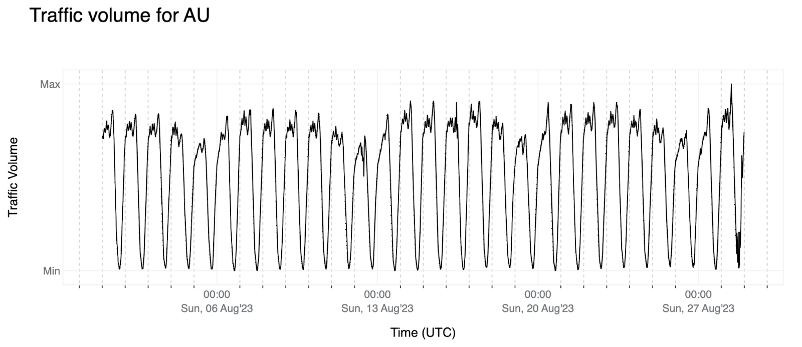
These statements can be clearly seen when we perform time-series decomposition which allows us to break down a time-series into its constituent parts to better understand and analyze its underlying patterns. Decomposing the traffic volume for Australia above assuming a weekly pattern with Seasonal-Trend decomposition using LOESS (STL) we get the following:

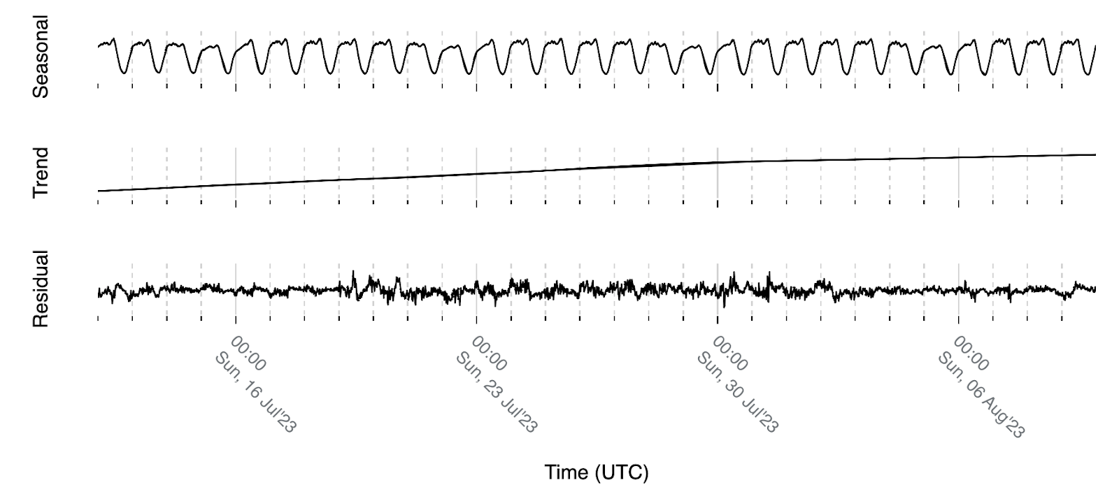
The weekly pattern we are referring to is represented by the seasonal part of the signal that is expected to be observed due to the fact that we are interested in eyeball / human internet traffic. As observed in the image above, the trend component is expected to move slowly when compared with the signal level and the residual part ideally would resemble white noise meaning that all existing patterns in the signal are represented by the seasonal and trend components.

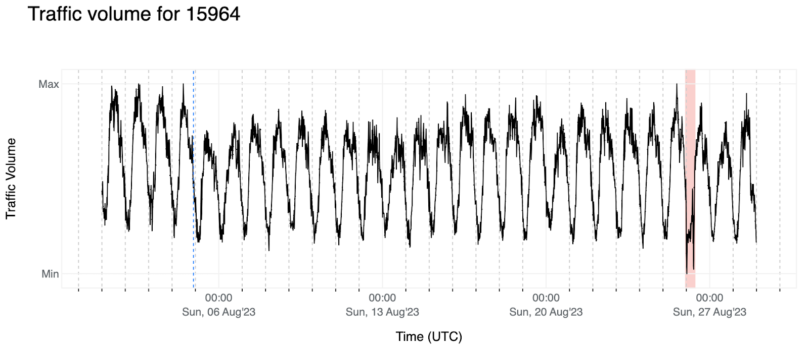
2. Below we have the traffic volume for AS15964 (CAMNET-AS) that appears to have more of a daily pattern, as opposed to weekly.

We also observe that there’s a value offset of the signal right after the first four days (blue dashed-line) and the red background shows us an outage for which we didn’t find any reporting besides seeing it in our data and other Internet data providers — our intention here is to develop an algorithm that will trigger an event when it comes across this or similar patterns.

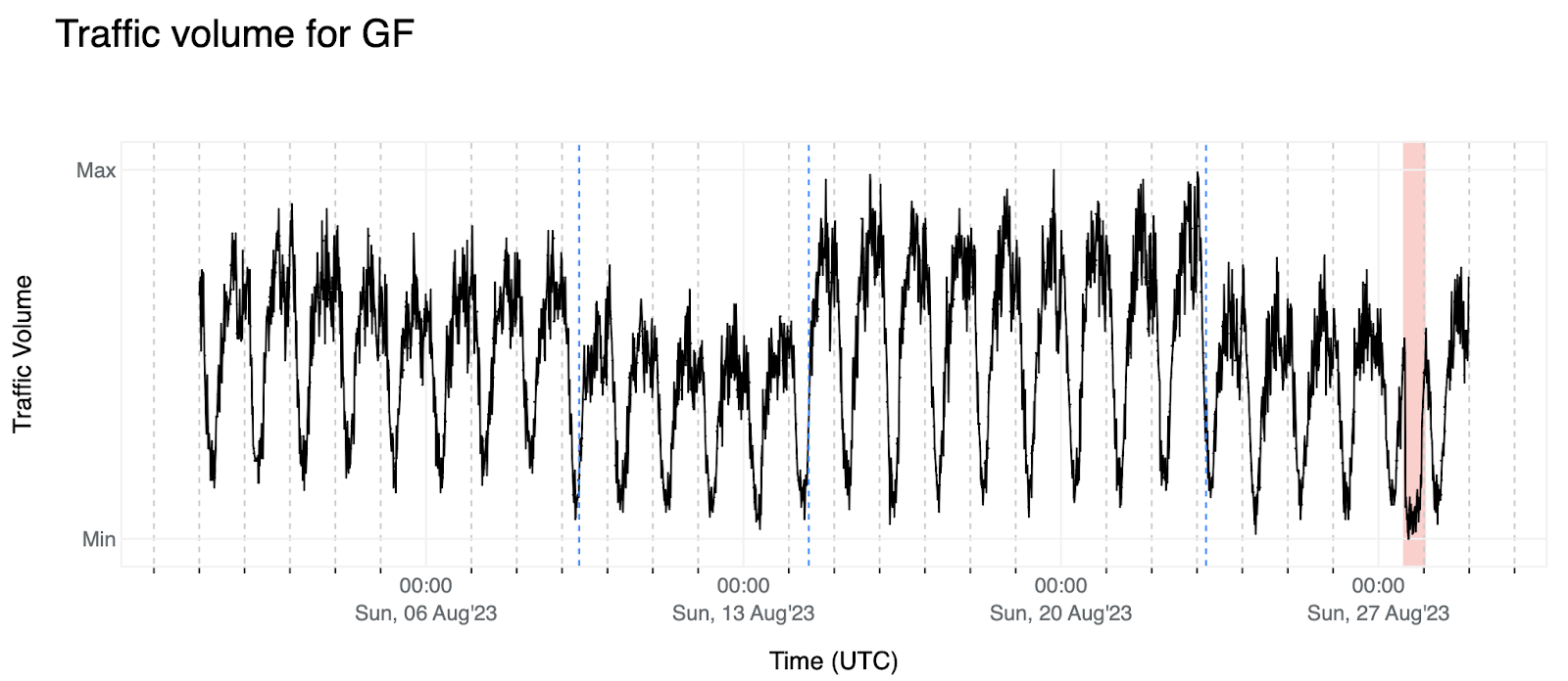
3. Here we have a similar example for French Guiana (GF). We observe some data offsets (August 9 and 23), a change in the amplitude (between August 15 and 23) and another outage for which we do have context that is observable in Cloudflare Radar.

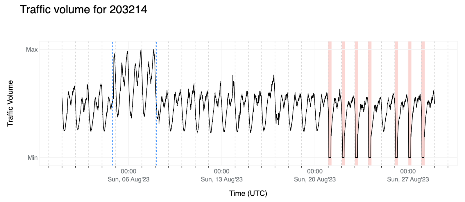
4. Another scenario is several scheduled outages for AS203214 (HulumTele), for which we also have context. These anomalies are the easiest to detect since the traffic goes to values that are unique to outages (cannot be mistaken as regular traffic), but it poses another challenge: if our plan was to just check the weekly patterns, since these government-directed outages happen with the same frequency, at some point the algorithm would see this as expected traffic.

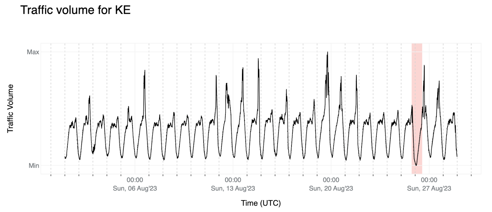
5. This outage in Kenya could be seen as similar to the above: the traffic volume went down to unseen values although not as significantly. We also observe some upward spikes in the data that are not following any specific pattern — possibly outliers — that we should clean depending on the approach we use to model the time-series.

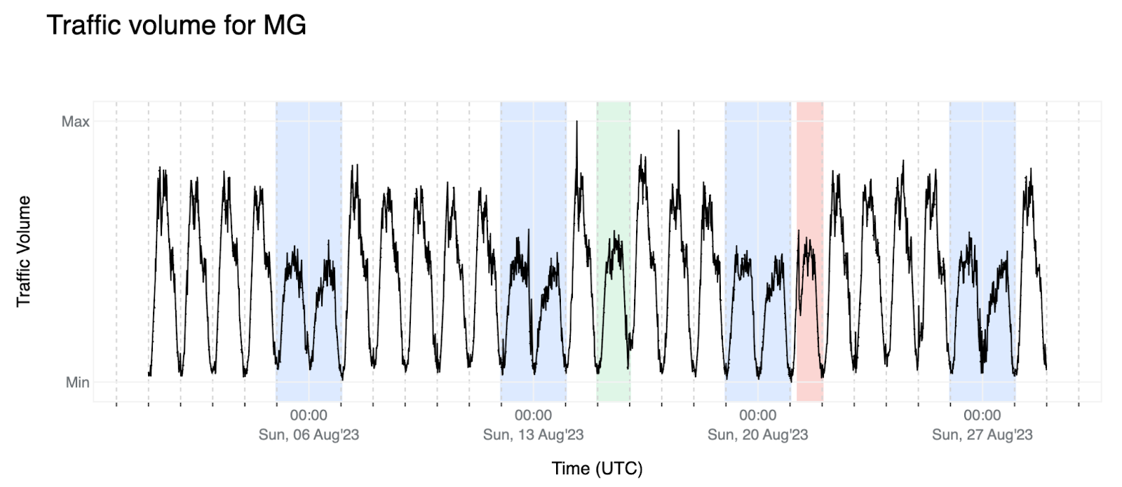
6. Lastly, here's the data that will be used throughout this post as an example of how we are approaching this problem. For Madagascar (MG), we observe a clear pattern with pronounced weekends (blue background). There’s also a holiday (Assumption of Mary), highlighted with a green background, and an outage, with a red background. In this example, weekends, holidays, and outages all seem to have roughly the same traffic volume. Fortunately, the outage gives itself away by showing that it intended to go up as in a normal working day, but then there was a sudden drop — we will see it more closely later in this post.

In summary, here we looked over six examples out of ~700 (the number of entities we are automatically detecting anomalies for currently) and we see a wide range of variability. This means that in order to effectively model the time-series we would have to run a lot of preprocessing steps before the modeling itself. These steps include removing outliers, detecting short and long-term data offsets and readjusting, and detecting changes in variance, mean, or magnitude. Time is also a factor in preprocessing, as we would also need to know in advance when to expect events / holidays that will push the traffic down, apply daylight saving time adjustments that will cause a time shift in the data, and be able to apply local time zones for each entity, including dealing with locations that have multiple time zones and AS traffic that is shared across different time zones.

To add to the challenge, some of these steps cannot even be performed in a close-to-real-time fashion (example: we can only say there’s a change in seasonality after some time of observing the new pattern). Considering the challenges mentioned earlier, we have chosen an algorithm that combines basic preprocessing and statistics. This approach aligns with our expectations for the data's characteristics, offers ease of interpretation, allows us to control the false positive rate, and ensures fast execution while reducing the need for many of the preprocessing steps discussed previously.

Above, we noted that we are detecting anomalies for around 700 entities (locations and autonomous systems) at launch. This obviously does not represent the entire universe of countries and networks, and for good reason. As we discuss in this post, we need to see enough traffic from a given entity (have a strong enough signal) to be able to build relevant models and subsequently detect anomalies. For some smaller or sparsely populated countries, the traffic signal simply isn’t strong enough, and for many autonomous systems, we see little-to-no traffic from them, again resulting in a signal too weak to be useful. We are initially focusing on locations where we have a sufficiently strong traffic signal and/or are likely to experience traffic anomalies, as well as major or notable autonomous systems — those that represent a meaningful percentage of a location’s population and/or those that are known to have been impacted by traffic anomalies in the past.

Detecting anomalies

The approach we took to solve this problem involves creating a forecast that is a set of data points that correspond to our expectation according to what we’ve seen in historical data. This will be explained in the section Creating a forecast. We take this forecast and compare it to what we are actually observing — if what we are observing is significantly different from what we expect, then we call it an anomaly. Here, since we are interested in traffic drops, an anomaly will always correspond to lower traffic than the forecast / expected traffic. This comparison is elaborated in the section Comparing forecast with actual traffic.

In order to compute the forecast we need to fulfill the following business requirements:

• We are mainly interested in traffic related to human activity.
• The more timely we detect the anomaly, the more useful it is. This needs to take into account constraints such as data ingestion and data processing times, but once the data is available, we should be able to use the latest data point and detect if it is an anomaly.
• A low False Positive (FP) rate is more important than a high True Positive (TP) rate. As an internal tool, this is not necessarily true, but as a publicly visible notification service, we want to limit spurious entries at the cost of not reporting some anomalies.

Selecting which entities to observe

Aside from the examples given above, the quality of the data highly depends on the volume of the data, and this means that we have different levels of data quality depending on which entity (location / AS) we are considering. As an extreme example, we don’t have enough data from Antarctica to reliably detect outages. Follows the process we used to select which entities are eligible to be observed.

For ASes, since we are mainly interested in Internet traffic that represents human activity, we use the number of users estimation provided by APNIC. We then compute the total number of users per location by summing up the number of users of each AS in that location, and then we calculate what percentage of users an AS has for that location (this number is also provided by the APNIC table in column ‘% of country’). We filter out ASes that have less than 1% of the users in that location. Here’s what the list looks like for Portugal — AS15525 (MEO-EMPRESAS) is excluded because it has less than 1% of users of the total number of Internet users in Portugal (estimated).

At this point we have a subset of ASes and a set of locations (we don’t exclude any location a priori because we want to cover as much as possible) but we will have to narrow it down based on the quality of the data to be able to reliably detect anomalies automatically. After testing several metrics and visually analyzing the results, we came to the conclusion that the best predictor of a stable signal is related to the volume of data, so we removed the entities that don’t satisfy the criteria of a minimum number of unique IPs daily in a two weeks period — the threshold is based on visual inspection.

Creating a forecast

In order to detect the anomalies in a timely manner, we decided to go with traffic aggregated every fifteen minutes, and we are forecasting one hour of data (four data points / blocks of fifteen minutes) that are compared with the actual data.

After selecting the entities for which we will detect anomalies, the approach is quite simple:

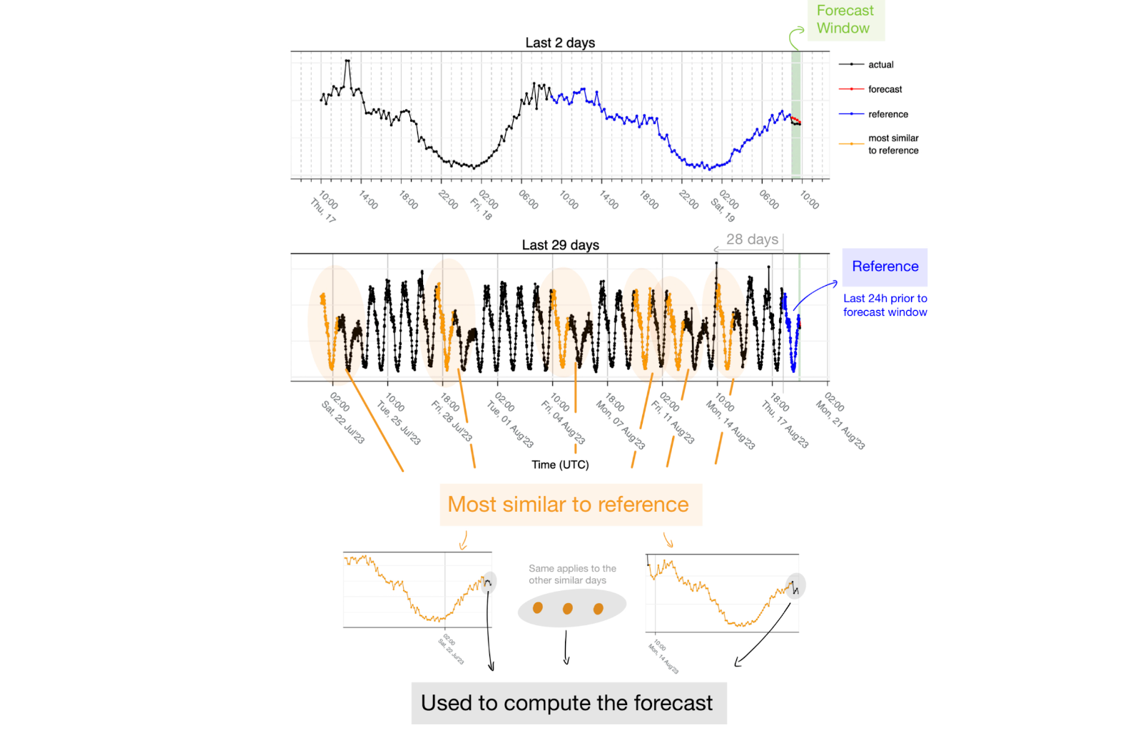
1. We look at the last 24 hours immediately before the forecast window and use that interval as the reference. The assumption is that the last 24 hours will contain information about the shape of what follows. In the figure below, the last 24 hours (in blue) corresponds to data transitioning from Friday to Saturday. By using the Euclidean distance, we get the six most similar matches to that reference (orange) — four of those six matches correspond to other transitions from Friday to Saturday. It also captures the holiday on Monday (August 14, 2023) to Tuesday, and we also see a match that is the most dissimilar to the reference, a regular working day from Wednesday to Thursday. Capturing one that doesn't represent the reference properly should not be a problem because the forecast is the median of the most similar 24 hours to the reference, and thus the data of that day ends up being discarded.

2. There are two important parameters that we are using for this approach to work:
   • We take into consideration the last 28 days (plus the reference day equals 29). This way we ensure that the weekly seasonality can be seen at least 4 times, we control the risk associated with the trend changing over time, and we set an upper bound to the amount of data we need to process. Looking at the example above, the first day was one with the highest similarity to the reference because it corresponds to the transition from Friday to Saturday.
   • The other parameter is the number of most similar days. We are using six days as a result of empirical knowledge: given the weekly seasonality, when using six days, we expect at most to match four days for the same weekday and then two more that might be completely different. Since we use the median to create the forecast, the majority is still four and thus those extra days end up not being used as reference. Another scenario is in the case of holidays such as the example below:

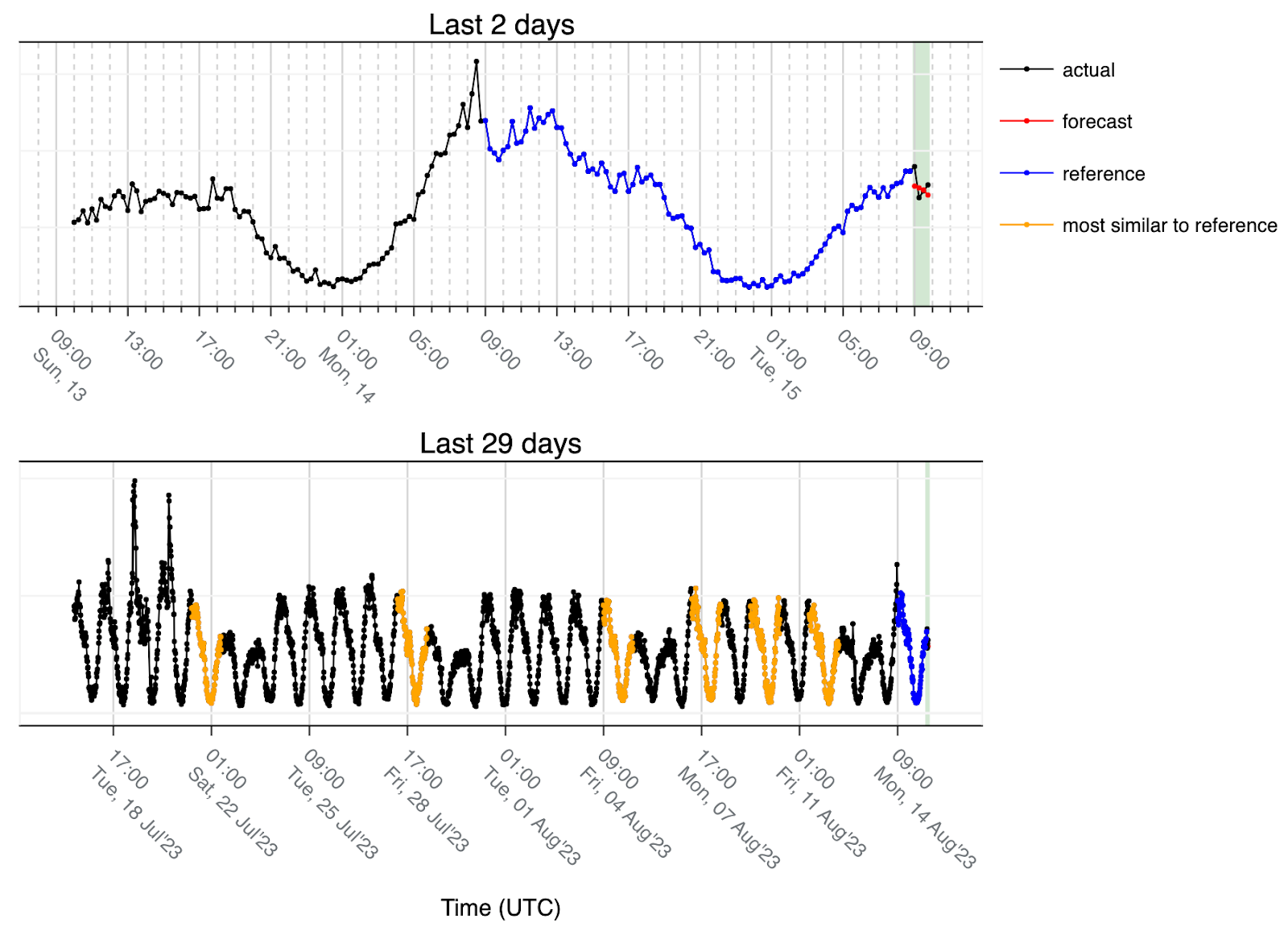
A holiday in the middle of the week in this case looks like a transition from Friday to Saturday. Since we are using the last 28 days and the holiday starts on a Tuesday we only see three such transitions that are matching (orange) and then another three regular working days because that pattern is not found anywhere else in the time-series and those are the closest matches. This is why we use the lower quartile when computing the median for an even number of values (meaning we round the data down to the lower values) and use the result as the forecast. This also allows us to be more conservative and plays a role in the true positive/false positive tradeoff.

Lastly let's look at the outage example:

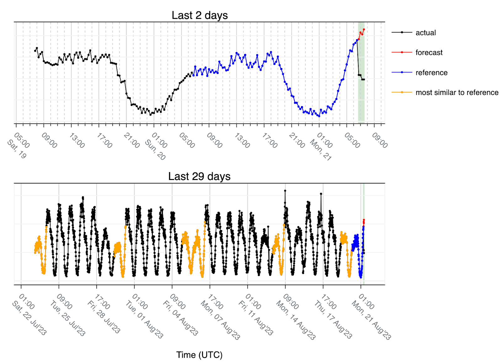
In this case, the matches are always connected to low traffic because the last 24h (reference) corresponds to a transition from Sunday to Monday and due to the low traffic the lowest Euclidean distance (most similar 24h) are either Saturdays (two times) or Sundays (four times). So the forecast is what we would expect to see on a regular Monday and that’s why the forecast (red) has an upward trend but since we had an outage, the actual volume of traffic (black) is considerably lower than the forecast.

This approach works for regular seasonal patterns, as would several other modeling approaches, and it has also been shown to work in case of holidays and other moving events (such as festivities that don’t happen at the same day every year) without having to actively add that information in. Nevertheless, there are still use cases where it will fail specifically when there’s an offset in the data. This is one of the reasons why we use multiple data sources to reduce the chances of the algorithm being affected by data artifacts.

Below we have an example of how the algorithm behaves over time.

Comparing forecast with actual traffic

Once we have the forecast and the actual traffic volume, we do the following steps.

We calculate relative change, which measures how much one value has changed relative to another. Since we are detecting anomalies based on traffic drops, the actual traffic will always be lower than the forecast.

After calculating this metric, we apply the following rules:

• The difference between the actual and the forecast must be at least 10% of the magnitude of the signal. This magnitude is computed using the difference between 95th and 5th percentiles of the selected data. The idea is to avoid scenarios where the traffic is low, particularly during the off-peaks of the day and scenarios where small changes in actual traffic correspond to big changes in relative change because the forecast is also low. As an example:
  • a forecast of 100 Gbps compared with an actual value of 80 Gbps gives us a relative change of -0.20 (-20%).
  • a forecast of 20 Mbps compared with an actual value of 10 Mbps gives us a much smaller decrease in total volume than the previous example but a relative change of -0.50 (50%).
• Then we have two rules for detecting considerably low traffic:
  • Sustained anomaly: The relative change is below a given threshold α throughout the forecast window (for all four data points). This allows us to detect weaker anomalies (with smaller relative changes) that are extended over time.

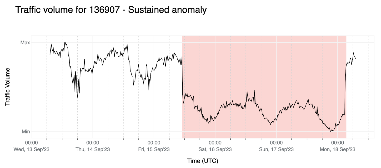
• Point anomaly: The relative change of the last data point of the forecast window is below a given threshold β (where β < α — these thresholds are negative; as an example, β and α might be -0.6 and -0.4, respectively). In this case we need β < α to avoid triggering anomalies due to the stochastic nature of the data but still be able to detect sudden and short-lived traffic drops.

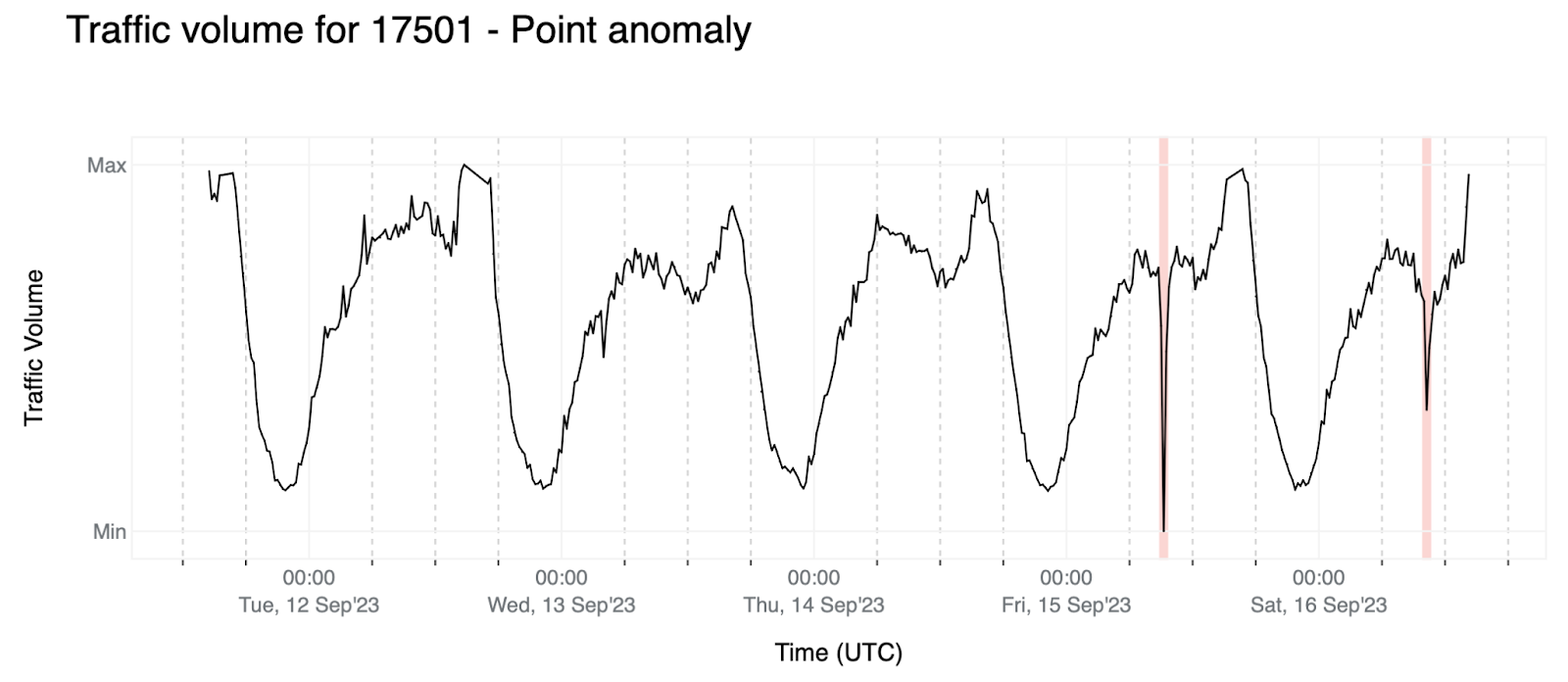
• The values of α and β were chosen empirically to maximize detection rate, while keeping the false positive rate at an acceptable level.

Closing an anomaly event

Although the most important message that we want to convey is when an anomaly starts, it is also crucial to detect when the Internet traffic volume goes back to normal for two main reasons:

• We need to have the notion of active anomaly, which means that we detected an anomaly and that same anomaly is still ongoing. This allows us to stop considering new data for the reference while the anomaly is still active. Considering that data would impact the reference and the selection of most similar sets of 24 hours.
• Once the traffic goes back to normal, knowing the duration of the anomaly allows us to flag those data points as outliers and replace them, so we don’t end up using it as reference or as best matches to the reference. Although we are using the median to compute the forecast, and in most cases that would be enough to overcome the presence of anomalous data, there are scenarios such as the one for AS203214 (HulumTele), used as example four, where the outages are frequently occurring at the same time of the day that would make the anomalous data become the expectation after few days.

Whenever we detect an anomaly we keep the same reference until the data comes back to normal, otherwise our reference would start including anomalous data. To determine when the traffic is back to normal, we use lower thresholds than α and we give it a time period (currently four hours) where there should be no anomalies in order for it to close. This is to avoid situations where we observe drops in traffic that bounce back to normal and drop again. In such cases we want to detect a single anomaly and aggregate it to avoid sending multiple notifications, and in terms of semantics there’s a high chance that it’s related to the same anomaly.

Conclusion

Internet traffic data is generally predictable, which in theory would allow us to build a very straightforward anomaly detection algorithm to detect Internet disruptions. However, due to the heterogeneity of the time series depending on the entity we are observing (Location or AS) and the presence of artifacts in the data, it also needs a lot of context that poses some challenges if we want to track it in real-time. Here we’ve shown particular examples of what makes this problem challenging, and we have explained how we approached this problem in order to overcome most of the hurdles. This approach has been shown to be very effective at detecting traffic anomalies while keeping a low false positive rate, which is one of our priorities. Since it is a static threshold approach, one of the downsides is that we are not detecting anomalies that are not as steep as the ones we’ve shown.

We will keep working on adding more entities and refining the algorithm to be able to cover a broader range of anomalies.

Visit Cloudflare Radar for additional insights around (Internet disruptions, routing issues, Internet traffic trends, attacks, Internet quality, etc.). Follow us on social media at @CloudflareRadar (Twitter), cloudflare.social/@radar (Mastodon), and radar.cloudflare.com (Bluesky), or contact us via e-mail.