Executive Summary

Unit 42 researchers discuss a machine learning pipeline we’ve built around memory-based artifacts from our hypervisor-based sandbox, which is part of Advanced WildFire. This alternative approach is one we’ve come up with to boost detection accuracy against malware using a variety of different evasion techniques.

As we discussed in our first two posts in this series, malware authors are routinely refining their shenanigans to make strategies like static analysis and sandboxing ineffective. The continual development and permutation of techniques like packing methodologies and sandbox evasions create a continual cat and mouse game that is difficult to stay on top of for any detection team.

To make matters worse, popular detection techniques such as structural analysis, static signatures and many types of dynamic analysis do not fare well against the ever-increasing complexity we encounter in the more prevalent malware families.

Table of Contents

Statically Armored and Full of Evasions
GuLoader Encrypted With NSIS Crypter
Why Static Analysis Isn’t Going To Help
NSIS Script and Extracting GuLoader Shellcode
Analysis of the Shellcode
Extracting Payload Information
How Can Machine Learning Detect This?
Detection Using Machine Learning
Feature Engineering
Model Selection
Training the Machine Learning Model
Interpreting Model Predictions
Interpreting Shapley Values
Finding Similar Samples Through Clustering
Conclusion
Indicators of Compromise
Additional Resources

Statically Armored and Full of Evasions

Malware authors increasingly employ evasion techniques such as obfuscation, packing and execution of dynamically injected shellcode in process memory. Using cues from the file structure for malware detection might not always succeed. Packing techniques modify the file structure sufficiently to eliminate these clues. Thus, machine learning models trained on this class of features alone would not effectively detect such samples.

Another popular alternative to this detection method is to use a machine learning model that predicts maliciousness based on the malware’s execution traces inside a sandbox. However, as detailed in our previous post in this series, sandbox evasions are extremely prevalent and payloads will often choose not to execute based on any number of clues that would point to a sample being emulated.

Malware can also inadvertently or intentionally corrupt the sandbox environment, overwrite log files or prevent successful analysis for any number of reasons due to the low-level tricks it is playing. This means that training our machine learning models on the execution logs is also not going to be enough to catch these evasive types of malware.

GuLoader Encrypted With NSIS Crypter

In this post, we will analyze one GuLoader downloader that has been encrypted with an Nullsoft Scriptable Install System (NSIS) crypter. NSIS is an open source system to create Windows installers.

Why Static Analysis Isn’t Going To Help

The GuLoader malware is encrypted, and it is also delivered through a NSIS installer file that is not ideal for static analysis because the file contents must be unpacked first. Once it’s unpacked, we are still left with encrypted data and one NSIS script. The script itself also dynamically decrypts some parts of the code, which is another factor that makes it harder to detect.

However, there are not many structural clues that would identify this as possible malware. Thus, a machine learning model trained on the Portable Executable (PE) file structure would not be effective in differentiating the file from other benign files.

NSIS Script and Extracting GuLoader Shellcode

To extract the NSIS script, we have to use an older version of 7-Zip, version 15.05. This version of 7-Zip is able to unpack the script, where newer versions have removed the functionality to unpack NSIS scripts. Once we have extracted the file contents and the NSIS script (shown in Figure 1), we can start analyzing the script and see how the GuLoader sample is being executed.

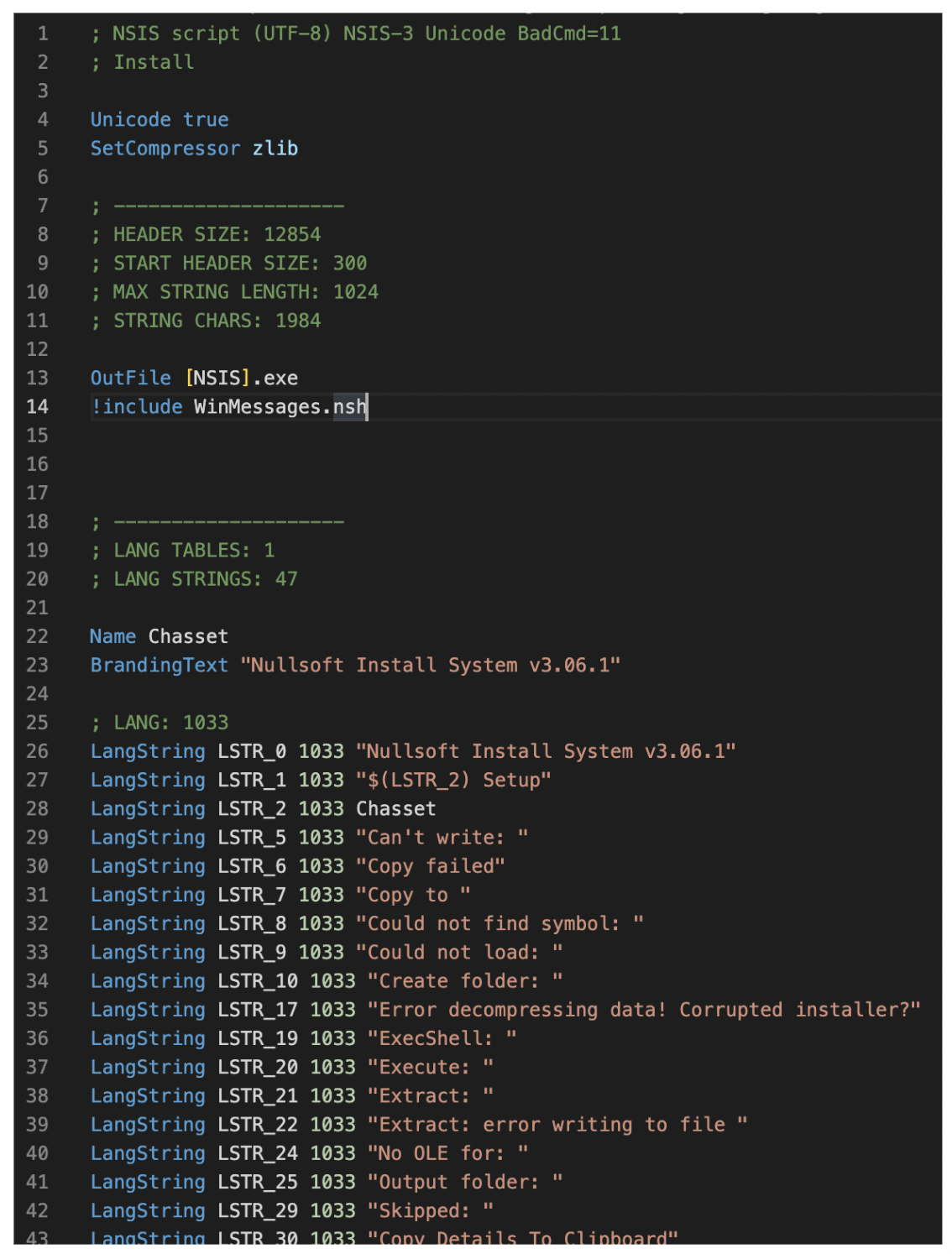
If we scroll down the script, we quickly notice that the files are being copied into a newly created folder named %APPDATA%\Farvelade\Skaermfeltet. Though it’s not clear why, the file paths used seem to be in Danish. After the copying activity, we have regular installation logic in the script, but there is one interesting function named func_30.

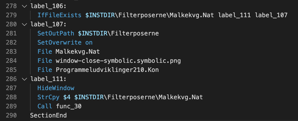
Before this function is called, the string $INSTDIR\Filterposerne\Malkekvg.Nat is copied into a string variable named $4, as shown in Figures 2 and 3. The function func_30 reads data from the Programmeludviklinger210.Kon file and builds up code, which it will call immediately after the character Z has been seen.

NSIS gives developers the ability to call any exported function from a Windows DLL, and it also allows developers to save the results directly in NSIS registers/stack. This functionality allows malware authors to dynamically call Windows API functions on runtime and makes static analysis harder because it must be evaluated before being analyzed.

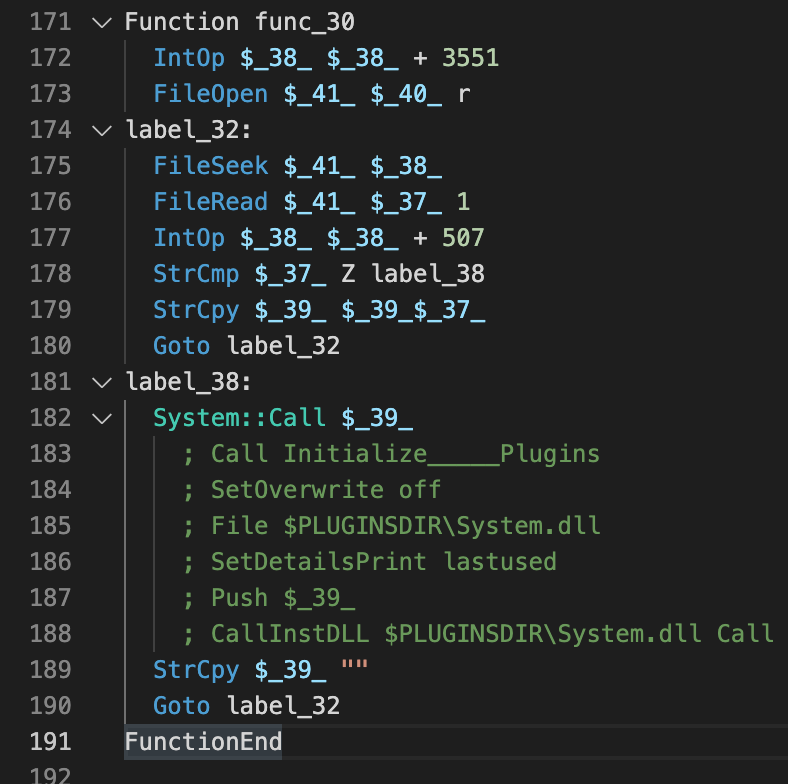
To decode the dynamic code, we can write a short Python script that reproduces the behavior and extracts the Windows API calls:

Figure 4 shows the decoded data that results from the script above.

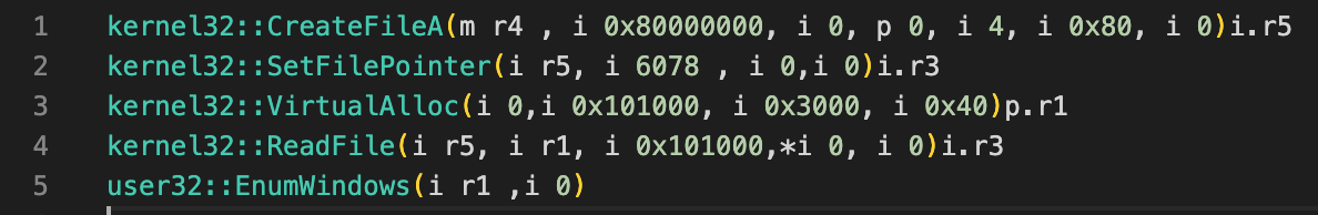
The decoded functions together read a shellcode from another file from the NSIS archive, and they execute it using the EnumWindows function. If we had to write this process in pseudo code, it would look something like this:

To make the remaining analysis easier, we are going to generate one PE with the shellcode. To generate the executable, we can either use a tool like Cerbero Profiler or LIEF Python library.

In this case, we have used the LIEF library to build a new executable. All we have to do is to add a new section with the contents of file Malkekvg.Nat and set the entry point to be at the correct offset. Once we get that, we should be able to open our shellcode in IDA Pro (shown in Figure 5) and see that it contains valid x86 instructions.

Analysis of the Shellcode

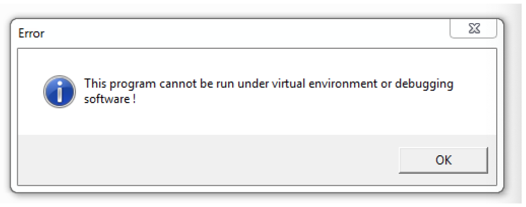
Now that we have the first stage of the shellcode inside a PE file we can run it in dynamic analysis and see what happens. The first thing that we will see is that it detects virtual machines and stops its execution after showing a message box. This text is decrypted on runtime using a 4-byte XOR key.

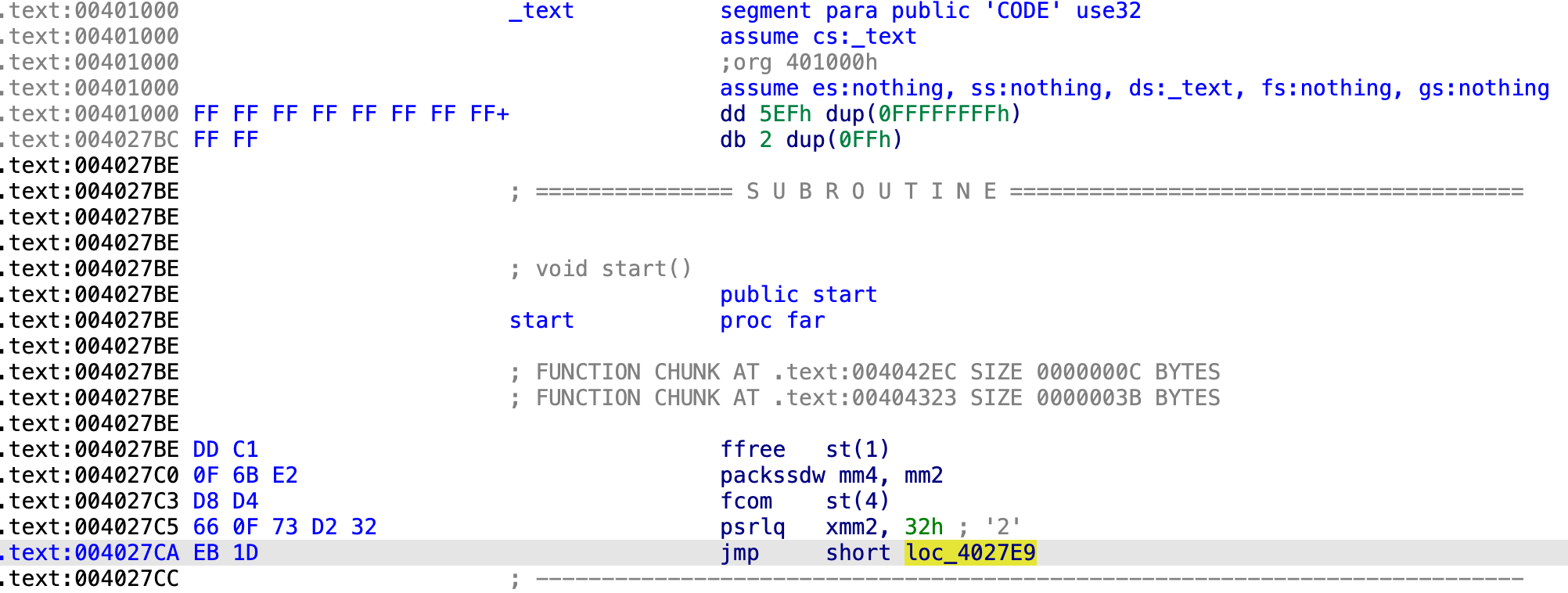
If we open the file in IDA Pro and follow the code a little, we should be able to see the large function for decrypting the first stage. While the function graph overview looks large, it’s still easy to identify junk code.

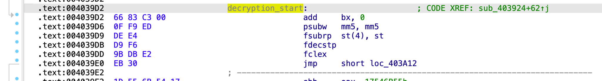
The code that is doing the decryption can be seen below in Figure 7. In Figure 8 we can see the final call that jumps to the second stage. At this point, we can dump the second stage into another executable for decryption.

We can dump the executable directly from memory, but we must make sure to patch the entry point to point to the correct address (which is 0x404328 in this example).

The second stage uses many anti-analysis techniques, which would be too long to describe here and are described elsewhere, so we won’t go too much detail. Here are a few of the anti-analysis techniques mentioned:

• Memory scan for known sandbox strings
• Hypervisor checks
• Time measuring
• Instruction hammering

To get the final payload that is being downloaded by GuLoader, we would have to either manually bypass all these checks, run it inside a sandbox that is immune to all of these techniques, or run it on a bare-metal sandbox.

Extracting Payload Information

To get the payload information (including all the strings) without analyzing the second stage, we can use a little trick that has been described by Spamhaus. GuLoader uses simple XOR encryption for encrypting its strings, which includes the payload URL.

All we need is the encryption key to decrypt everything. The good news is that the key resides somewhere inside the second stage.

To decrypt the strings, we can use brute-force on a pattern that we already know exists inside the second stage. The result of that XOR operation would be our key. The only limitation to this is that the pattern must be large enough so that we are able to fully decrypt the payload URL. For example, a good pattern might be the user-agent string, which is set by default to Mozilla/5.0 (Windows NT 10.0; WOW64; Trident/7.0; rv:11.0) like Gecko.

To quickly find the decryption key automatically, we have to encrypt a short pattern first (e.g., first 8 bytes of the user-agent string) and search if that result is somewhere in the file. If it is somewhere in the file, then we can continue and encrypt the remaining pattern to get the full encryption key.

At the end of this blog, we have attached the Python script that is able to find the encryption key from the payload by the method described above. Once we run the script on any dumped second stage GuLoader payload, we should be able to see a few strings and the payload URL.

GuLoader sometimes includes 7 to 8 random characters in front of the payload URL, which it replaces on runtime with either http:// or https://. The distinction of whether http or https is used is made by the fourth character from that random pattern.

In this sample, the payload URL was http://ozd[.]com[.]ar/wp-includes/nHMoYlbGLWls101.qxd and the payload was still online at the time of this analysis.

The final downloaded payload is from the FormBook malware family, and it had the SHA256 value of fa0b6404535c2b3953e2b571608729d15fb78435949037f13f05d1f5c1758173.

How Can Machine Learning Detect This?

In a previous blog post, we detailed several types of observable artifacts that we can extract from memory during a live sandbox run. We’ve found that the data from memory analysis is extremely powerful when combined with machine learning for the detection of malware with multiple evasion techniques.

The following section describes our strategy for taking all these observations about what was modified in memory at runtime and combining them with machine learning at scale for malware detection. The algorithm can find patterns automatically, and it can identify commonalities that indicate when malware is attempting to hide its footprints in memory, dynamically allocating and executing shell code, or using unpacking.

In this GuLoader sample, right off the bat, a human analyst would identify that there are a few unique function pointers. We would also notice that the malware has changed the page permissions of multiple pages in its own process memory to writable and executable. Our machine learning model is able to automatically perform these activities, taking the features extracted from the various memory artifacts to detect the GuLoader sample.

As we discussed earlier in this blog series, the automated analysis platform we’ve created for Advanced WildFire will automatically extract all of these memory-based artifacts in a performant way. This means that all of the information related to dynamically resolved function pointers, permissions changes and unpacked executables can be utilized either in our manually curated detection logic or additionally for our machine learning pipelines.

Detection Using Machine Learning

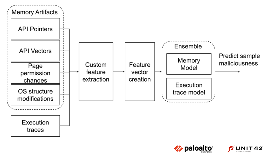
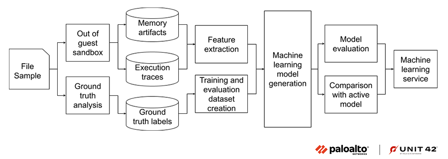
Figure 9 shows a high level view of how we created a machine learning model pipeline trained on custom features extracted from the aforementioned memory-based artifacts. The features we chose were fashioned to retain the most useful information from the verbose artifacts.

We also included malware execution traces as an extra source of information and built an ensemble model to detect the malicious samples. As shown in Figure 9 below, various custom features are automatically extracted from the four memory artifacts and malware execution traces, and they are passed to a classification model for detecting malicious samples. Furthermore, we have built an ensemble model that is trained on memory artifacts and execution trace based features to boost its performance.

Feature Engineering

We’ve experimented with the efficacy of raw values from the different feature sources versus custom features for the purposes of model accuracy. Using custom features built using domain knowledge enables us to reduce noise and minimize the number of features overall, thus helping avoid the curse of dimensionality.

At the same time, using raw values as features allows us to quickly adapt to newer malware trends that might use changing attack tactics and techniques. We have utilized deep learning to extract features from the logs involving extracted memory-based artifacts and combine that with custom features. Our experiments show that the models work best with a combination of the two approaches.

Model Selection

When it comes to model selection, there are a few factors that we have to consider:

• Small model size allows for scaling up the machine learning service to accommodate the ever growing number of samples to process.
• Account for the absence of certain feature sources, (e.g., execution traces) in case of errors encountered.
• Model predictions should be interpretable so we can identify the causal features in the case of disruptive false positives.
• The model should attempt to retain as much information as possible from the samples it has trained on.

A gradient-boosted trees model trained on domain-specific features and custom features extracted from raw data satisfies many of the aforementioned criteria.

Training the Machine Learning Model

The file samples are processed by a streaming pipeline to save memory artifacts and other malware attributes to a feature store. The feature extraction stage uses a combination of streaming and batch processing PySpark jobs to generate the final feature vector used for training the model.

The ground truth labels come from a separate pipeline that assigns labels to the samples based on malware characteristics and researcher inputs. The pipeline generates non-overlapping training and evaluation datasets by using the sample first seen time and hashes.

Once the machine learning model is trained and satisfies the predefined evaluation checks, including expected improvement over the currently active model, it’s pushed to the production machine learning service.

Interpreting Model Predictions

It’s crucial to understand the machine learning model’s predictions in order to identify the limitations and the capabilities of the model. Machine learning is prone to false positives, as it’s heavily dependent on the quality and variety of the training data, as well as the ability to generalize on a changing landscape of files to predict on. Thus, having the ability to identify the causal features for a prediction can be very helpful.

We use two methodologies to assist with this process.

Interpreting Shapley Values

Shapley Additive Explanations (SHAP) is a game-theoretical approach used to explain the output of any machine learning model. The SHAP values explain the influence of each feature on the actual prediction for an input feature vector as opposed to the baseline prediction. In Figure 11, the features in red, from right to left, are the topmost features that push the model towards a malicious prediction. The features in blue, from left to right, indicate the topmost features that reduce the probability of the prediction being malware.

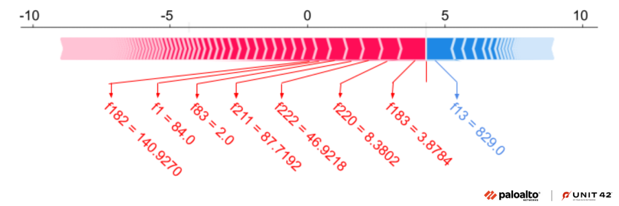
In the figure above, we have plotted the force plot for the top seven features with significant SHAP values and their corresponding raw feature values. Our machine learning model was able to detect GuLoader due to the presence of these top features. These features correspond to several specific dynamically resolved API pointers and their relative locations in memory, as well as the relative types of memory page permission changes that were made by the sample.

Finding Similar Samples Through Clustering

Another approach to understanding the model’s predictions is to identify similar samples in the training dataset. We use density based scan (DBScan) as a clustering technique, shown in Figure 12, as it allows for outliers and different shaped clusters.

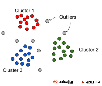
This approach also expands its use beyond model interpretation to find similar samples that belong to the same malware family or APT group. Using DBScan we can find out the cluster where the GuLoader sample resides and extract samples. Furthermore, we can also extract samples which are similar to it in feature space.

Conclusion

The GuLoader family is an excellent example of malware to detect with our machine learning model, because its use of sandbox evasions and static armoring makes it hard for traditional defenses to detect using structural cues and execution logs alone.

With Advanced WildFire, we introduce a hypervisor-based sandbox that can stealthily observe the memory of GuLoader during execution to parse meaningful memory resident artifacts and information useful for our machine learning detection pipeline. This allows us to accurately detect the malicious behavior using features extracted from the observed memory-based artifacts.

Palo Alto Networks customers receive protections from threats such as those discussed in this post with Advanced WildFire.

Indicators of Compromise

cc6860e4ee37795693ac0ffe0516a63b9e29afe9af0bd859796f8ebaac5b6a8c
fa0b6404535c2b3953e2b571608729d15fb78435949037f13f05d1f5c1758173 (Final payload)

Additional Resources

Threat Assessment: GandCrab and REvil Ransomware
SHAP Documentation
GuLoader Strings Decryptor