In my old article I have demonstrated an atypical approach one may take to browse through similarly-looking security artifacts while analyzing a gazillion of similarly looking URls in Excel.

I love Excel and been using it for more than 2 decades. It is one of these ‘most important’ but often undervalued tools in our infosec toolkit that we all have an opinion about: we either love it or hate it. And – I must confess that my opinion is supported by what I have witnessed in many different companies over the years – it often feels that to many Excel users, including infosec pros, some of its functionality is not only remotely unfamiliar — it is actually absolutely unknown!

Why don’t we change that!?

Here we are in year 2023… Excel is all over the place, whether as an email attachment (this time non-malicious!), or a shared document, whether helping us with a snapshot of forensic evidence, opening a CSV/XLSX export from Splunk, or other platforms, or is being used by DFIR or compliance folks, or even more often – by all these security committees and security project managers that like to push paper, and all this feels good, but… while so many of us and them use it, not so many of us and them know or are eager to explore ways to know it better…

What makes Excel an excellent tool for security people?

How about a streamlined way for… data import, data conversion, data sorting, data filtering, data reduction, data normalization, data extraction, data transformations, algorithmic data processing and then an ability to present this data and processing results in not only many ways possible, but also the ease of doing so (using pivot tables, charts, filters, and many other options available). We simply need to invest time to understand this tool better.

The article I linked to was about using VBA — this, for many, is an advanced level. Let’s come closer to the basics: dates, formulas, formatting.

One of the easiest way to demonstrate Excel’s power it building a self-formatting timeline. I have used this approach (a template really) in one or another form for many different cases, not only in forensics, but also for planning, and scheduling. And once you create it manually, at least once, you will find it very tempting to use it for many different projects in the future…

Let’s begin (steps are Windows-centric, but for most of the steps Ctrl->CMD switch on macOS will suffice).

Create a new workbook and go to A1 cell. Type =NOW() and press Enter. You should see something like this:

You can save it as foo.xlsx, or whatever. The A1 cell will always hold the value of a current time. So, anytime you open this Excel file, it will be there, in A1, up to date.

Copy the content of this A1 cell (Ctrl+C), and then Paste it Special into B1 – using the options from a dialog box that pops up, paste it as a value (CTRL+ALT+V, ALT+H+V+S).

You may see something like this:

Note that the time in A1 has already changed. It doesn’t matter for this exercise.

The B1 contains a number. This is how Excel stores info about the date. We can add meaning to it by formatting it as a date. You can use Format Painter, click it while in A1, and then apply it to B1:

The time in A1 has changed again, but B1 is now fixed (because it’s a value, not a formula).

Go to B1, and Press Ctrl+1. You will see the Format Cell Dialog Box. Go to Custom and Type YYYY-MM-DD (ddd), then hit Enter to see the dateish number being reformatted to a date:

We now have a ‘starting’ date for our timeline, formatted in a proper way.

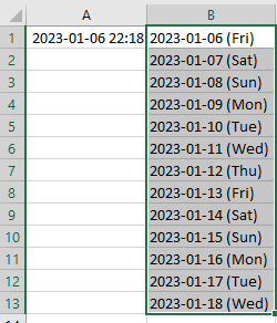
Go to B2, and type =B1+1 and then hit Enter. And once you do it, you will see:

That is the beginning of our timeline.

While in B2, press SHIFT and go a few rows down, then press CTRL+D. This will populate the very same formula (B1+1) down, of course, adjusting it to use a preceding row’s cell as a point of reference:

We can format it to the left so it looks neater:

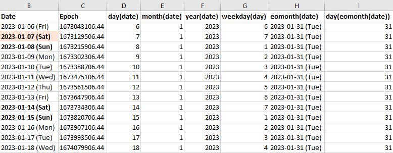
It’s time to extract some properties from the list of dates we have created. We add column headers first (for readability) and then make their text bold so at least we have a point of reference for what the formulas in each column extract. Then we try to add a bunch of formulas in row 2 – by typing formulas as shown on the below pic (look at the second row only and type these in your sheet; you will populate the next rows automagically via CTRL+D):

Column B1 is an initial date we copied from A1 (preserved as a value; and in a way Excel stores dates; followed by ‘plus 1’ formulas in subsequent rows), and then formulas in C, D, E, F, G, H are as follows:

• day – extracts a day from a given date
• month – extracts a month from a given date
• year – extracts a year from a given date
• weekday – extract number representing ‘day of the week’ i.e. Sun (1), Mon (2), Tue (3), Wed (4), Thu (5), Fri (6), Sat (7)
• eomonth – tells us what is the last date of the month we are currently in
• day(eomonth) – as above, except it just tells us the day only

Once we put these in, we then use SHIFT and use a selection with cursors (covering multiple columns), then press CTRL+D to populate formulas to apply to the next dates below (next rows); we should be seeing these values now:

Hint: at anytime, you can use CTRL+` to switch between formulas and data/values view.

The main purpose of extracting these properties is to use them later in our Conditional Formatting rules. These are pretty useful rules applied per cell, or group of cells and adding extra readability features to the ‘presentation layer’ for the data we are seeing/processing/looking at.

For instance, if we want Saturday and Sunday to be marked as bold, we can select the column B and apply the following Conditional Formatting rule:

It basically means: if the day of the week for a current date is 1 (Sun) or 7 (Sat), mark it bold. Which, when applied, gives us this result:

We can add additional Conditional Formatting rule that will ‘highlight light red’ the current date (that is, happening ‘today’):

And we can add a few more rows, covering the whole month, plus more. With this test data in place we can now use the value of the column H which indicates what is the last day of the current date’s month. Using this value we can add additional conditional formatting showing a ‘separator’ line after the last day of the month:

So, these are basics for a generic timeline/date-oriented ‘layout’ one can easily produce in Excel for any kinda of data really. While the example focuses on days only (YYYY-MM-DD (ddd)) which is very handy for day-to-day diaries, long-term-project scheduling, and multi-regional, follow-the-Sun scheduling, it’s very easy to expand it to more ‘forensicish’ timelines including hours, minutes, seconds and smaller time intervals. For Forensic cases, I find it particularly useful to combine many logs from many sources and (after normalizing them all to UTC) mapping them out on a single, unified timeline: and it’s always possible to add many artifacts to this timeline:

• file-system (creation, modification, access, etc.)
• process timelines (process creation, end, etc.)
• embedded timestamps f.ex. PE Clustering
• web-logs
• error-logs
• any other network logs
• any user or system activities reported externally, elsewhere
• etc.

Adding additional timezones or epoch is also easy, f.ex. using this Excel timestamp to Epoch formula:

=(B2-DATE(1970,1,1))*86400

we can create an additional column showing us timestamps in a familiar, Epoch way:

The same goes with other timezones — very easy, very straight forward, easy to normalize timezones and accompanying data.

Are there better tools to do it? I hope… yes. But. Excel works with a raw data and gives us an opportunity to VALIDATE results provided by other tools. Plus, full control gives us no excuses when it comes to an interpretation of evidence.